Convolutional neural networks
Contents
10.2. Convolutional neural networks
Convolutional neural networks (CNNs) are a type of neural network that are particularly well-suited for images, in computer vision tasks including image classification, object detection, and image segmentation. The main idea behind CNNs is to use a convolutional layer to extract features from the image locally. The convolutional layer is typically followed by a pooling layer to reduce the dimensionality. The convolutional and pooling layers are then followed by one or more fully connected layers, e.g. to classify the image.
On 30 September 2012, a CNN called AlexNet (click to view the architecture) achieved a top-5 error of 15.3% in the ImageNet Challenge, more than 10.8 percentage points lower than that of the runner up. This is considered a breakthrough and has grabbed the attention of increasing number of researchers, practitioners, and the general public. Since then, deep learning has penetrated to many research and application areas. AlexNet contained eight layers. In 2015, it was outperformed by a very deep CNN with over 100 layers from Microsoft in the ImageNet 2015 contest.
Watch the 14-minute video below for a visual explanation of convolutional neural networks.
Video
Explaining main ideas behind convolutional neural networks by StatQuest, embedded according to YouTube’s Terms of Service.
Remove or comment off the following installation if you have installed PyTorch and TorchVision already.
!pip3 install -q torch torchvision
[notice] A new release of pip is available: 23.0.1 -> 24.0
[notice] To update, run: pip install --upgrade pip
10.2.1. Why convolutional neural networks?
In the previous section, we used fully connected neural networks to classify digit images, where the input image needs to be flattened into a vector. There are two major drawbacks of using fully connected neural networks for image classification:
The number of parameters in the fully connected layer can be very large. For example, if the input image is \(28\times 28\) pixels (MNIST), then the number of weights for each hidden unit in the fully connected layer is \(28\times 28 = 784\). If the number of hidden units in the fully connected layer is 100, then the number of weight parameters in the fully connected layer is \(784\times 100 = 78,400\), for a total of \(78,400 + 100 = 78,500\) parameters (there are 100 bias parameters). If we have an input image of a larger size \(224\times 224\) pixels, then the total number of parameters in the fully connected layer with 100 hidden units is \(224\times 224 \times 100 + 100 = 5,017,700\). This is a lot of parameters to learn and to compute the output once the network is trained.
Fully connected neural networks do not make use of the spatial structure of the image. Moreover, a small shift in the position of the image can result in a very different input vector and thus the output of the network can be quite different. This is not desirable for image classification. For image classification, we hope to utilise and preserve the spatial information of the image. This is where convolutional neural networks come in.
There are two key ideas behind convolutional neural networks:
Local connectivity: The convolutional layer is only connected to a small region of the input. This allows the convolutional layer to learn local features using only a small number of parameters.
Weight sharing: The weights in the convolutional layer are shared across the entire input to detect the same local feature at different locations, across the entire input. This greatly reduces the number of parameters to learn.
Let us see how convolutional neural networks work on an example of image classification adapted from the PyTorch tutorial Training a classifier and the CNN notebook from Lisa Zhang
10.2.2. Load the CIFAR10 image data
Get ready by importing the APIs needed from respective libraries and setting the random seed for reproducibility.
import numpy as np
import torch
import torch.nn as nn
import torch.nn.functional as F
import torch.optim as optim
import torchvision
from torchvision import datasets, transforms
import matplotlib.pyplot as plt

%matplotlib inline

torch.manual_seed(2022)
np.random.seed(2022)
It will be good to be aware of the version of PyTorch and TorchVision you are using. The following code will print the version of PyTorch and TorchVision. This notebook is developed using PyTorch 1.13.1 and TorchVision 0.14.1.
torch.__version__
'2.2.0+cu121'
torchvision.__version__
'0.17.0+cu121'
The CIFAR10 dataset has ten classes: ‘airplane’, ‘automobile’, ‘bird’, ‘cat’, ‘deer’, ‘dog’, ‘frog’, ‘horse’, ‘ship’, ‘truck’. The images in CIFAR-10 are of size \(3\times 32\times 32\), i.e. 3-channel colour images of \(32\times 32\) pixels in size.
As in the case of MNIST, the torchvision package has a data loader for CIFAR10 as well. The data loader downloads the data from the internet the first time it is run and stores it in the given root directory.
Similar to the MNIST example, we apply the ToTensor transform to convert the PIL images to tensors. In addition, we also apply the Normalize transform to normalise the images with some preferred mean and standard deviation, such as (0.5, 0.5, 0.5) and (0.5, 0.5, 0.5) used below or the mean and standard deviation of the ImageNet dataset (0.485, 0.456, 0.406) and (0.229, 0.224, 0.225) respectively.
Let us load the train and test sets using a batch size of 8, i.e. each element in the dataloader train_loader is a list of 8 images and their corresponding labels. The num_workers argument specifies the number of subprocesses to use for data loading. We use 2 subprocesses here for faster data loading.
batch_size = 8
root_dir = "./data"
transform = transforms.Compose(
    [transforms.ToTensor(), transforms.Normalize((0.5, 0.5, 0.5), (0.5, 0.5, 0.5))]
)

train_dataset = datasets.CIFAR10(
    root=root_dir, train=True, download=True, transform=transform
)
test_dataset = datasets.CIFAR10(
    root=root_dir, train=False, download=True, transform=transform
)

train_loader = torch.utils.data.DataLoader(
    train_dataset, batch_size=batch_size, shuffle=True, num_workers=2
)
test_loader = torch.utils.data.DataLoader(
    test_dataset, batch_size=batch_size, shuffle=False, num_workers=2
)
0.0%
0.0%
0.1%
0.1%
0.1%
0.1%
0.1%
0.2%
0.2%
0.2%
0.2%
0.2%
0.2%
0.3%
0.3%
0.3%
0.3%
0.3%
0.4%
0.4%
0.4%
0.4%
0.4%
0.5%
0.5%
0.5%
0.5%
0.5%
0.6%
0.6%
0.6%
0.6%
0.6%
0.7%
0.7%
0.7%
0.7%
0.7%
0.7%
0.8%
0.8%
0.8%
0.8%
0.8%
0.9%
0.9%
0.9%
0.9%
0.9%
1.0%
1.0%
1.0%
1.0%
1.0%
1.1%
1.1%
1.1%
1.1%
1.1%
1.2%
1.2%
1.2%
1.2%
1.2%
1.2%
1.3%
1.3%
1.3%
1.3%
1.3%
1.4%
Downloading https://www.cs.toronto.edu/~kriz/cifar-10-python.tar.gz to ./data/cifar-10-python.tar.gz
1.4%
1.4%
1.4%
1.4%
1.5%
1.5%
1.5%
1.5%
1.5%
1.6%
1.6%
1.6%
1.6%
1.6%
1.7%
1.7%
1.7%
1.7%
1.7%
1.7%
1.8%
1.8%
1.8%
1.8%
1.8%
1.9%
1.9%
1.9%
1.9%
1.9%
2.0%
2.0%
2.0%
2.0%
2.0%
2.1%
2.1%
2.1%
2.1%
2.1%
2.2%
2.2%
2.2%
2.2%
2.2%
2.2%
2.3%
2.3%
2.3%
2.3%
2.3%
2.4%
2.4%
2.4%
2.4%
2.4%
2.5%
2.5%
2.5%
2.5%
2.5%
2.6%
2.6%
2.6%
2.6%
2.6%
2.7%
2.7%
2.7%
2.7%
2.7%
2.7%
2.8%
2.8%
2.8%
2.8%
2.8%
2.9%
2.9%
2.9%
2.9%
2.9%
3.0%
3.0%
3.0%
3.0%
3.0%
3.1%
3.1%
3.1%
3.1%
3.1%
3.2%
3.2%
3.2%
3.2%
3.2%
3.2%
3.3%
3.3%
3.3%
3.3%
3.3%
3.4%
3.4%
3.4%
3.4%
3.4%
3.5%
3.5%
3.5%
3.5%
3.5%
3.6%
3.6%
3.6%
3.6%
3.6%
3.7%
3.7%
3.7%
3.7%
3.7%
3.7%
3.8%
3.8%
3.8%
3.8%
3.8%
3.9%
3.9%
3.9%
3.9%
3.9%
4.0%
4.0%
4.0%
4.0%
4.0%
4.1%
4.1%
4.1%
4.1%
4.1%
4.2%
4.2%
4.2%
4.2%
4.2%
4.2%
4.3%
4.3%
4.3%
4.3%
4.3%
4.4%
4.4%
4.4%
4.4%
4.4%
4.5%
4.5%
4.5%
4.5%
4.5%
4.6%
4.6%
4.6%
4.6%
4.6%
4.7%
4.7%
4.7%
4.7%
4.7%
4.7%
4.8%
4.8%
4.8%
4.8%
4.8%
4.9%
4.9%
4.9%
4.9%
4.9%
5.0%
5.0%
5.0%
5.0%
5.0%
5.1%
5.1%
5.1%
5.1%
5.1%
5.2%
5.2%
5.2%
5.2%
5.2%
5.2%
5.3%
5.3%
5.3%
5.3%
5.3%
5.4%
5.4%
5.4%
5.4%
5.4%
5.5%
5.5%
5.5%
5.5%
5.5%
5.6%
5.6%
5.6%
5.6%
5.6%
5.7%
5.7%
5.7%
5.7%
5.7%
5.7%
5.8%
5.8%
5.8%
5.8%
5.8%
5.9%
5.9%
5.9%
5.9%
5.9%
6.0%
6.0%
6.0%
6.0%
6.0%
6.1%
6.1%
6.1%
6.1%
6.1%
6.2%
6.2%
6.2%
6.2%
6.2%
6.2%
6.3%
6.3%
6.3%
6.3%
6.3%
6.4%
6.4%
6.4%
6.4%
6.4%
6.5%
6.5%
6.5%
6.5%
6.5%
6.6%
6.6%
6.6%
6.6%
6.6%
6.6%
6.7%
6.7%
6.7%
6.7%
6.7%
6.8%
6.8%
6.8%
6.8%
6.8%
6.9%
6.9%
6.9%
6.9%
6.9%
7.0%
7.0%
7.0%
7.0%
7.0%
7.1%
7.1%
7.1%
7.1%
7.1%
7.1%
7.2%
7.2%
7.2%
7.2%
7.2%
7.3%
7.3%
7.3%
7.3%
7.3%
7.4%
7.4%
7.4%
7.4%
7.4%
7.5%
7.5%
7.5%
7.5%
7.5%
7.6%
7.6%
7.6%
7.6%
7.6%
7.6%
7.7%
7.7%
7.7%
7.7%
7.7%
7.8%
7.8%
7.8%
7.8%
7.8%
7.9%
7.9%
7.9%
7.9%
7.9%
8.0%
8.0%
8.0%
8.0%
8.0%
8.1%
8.1%
8.1%
8.1%
8.1%
8.1%
8.2%
8.2%
8.2%
8.2%
8.2%
8.3%
8.3%
8.3%
8.3%
8.3%
8.4%
8.4%
8.4%
8.4%
8.4%
8.5%
8.5%
8.5%
8.5%
8.5%
8.6%
8.6%
8.6%
8.6%
8.6%
8.6%
8.7%
8.7%
8.7%
8.7%
8.7%
8.8%
8.8%
8.8%
8.8%
8.8%
8.9%
8.9%
8.9%
8.9%
8.9%
9.0%
9.0%
9.0%
9.0%
9.0%
9.1%
9.1%
9.1%
9.1%
9.1%
9.1%
9.2%
9.2%
9.2%
9.2%
9.2%
9.3%
9.3%
9.3%
9.3%
9.3%
9.4%
9.4%
9.4%
9.4%
9.4%
9.5%
9.5%
9.5%
9.5%
9.5%
9.6%
9.6%
9.6%
9.6%
9.6%
9.6%
9.7%
9.7%
9.7%
9.7%
9.7%
9.8%
9.8%
9.8%
9.8%
9.8%
9.9%
9.9%
9.9%
9.9%
9.9%
10.0%
10.0%
10.0%
10.0%
10.0%
10.1%
10.1%
10.1%
10.1%
10.1%
10.1%
10.2%
10.2%
10.2%
10.2%
10.2%
10.3%
10.3%
10.3%
10.3%
10.3%
10.4%
10.4%
10.4%
10.4%
10.4%
10.5%
10.5%
10.5%
10.5%
10.5%
10.6%
10.6%
10.6%
10.6%
10.6%
10.6%
10.7%
10.7%
10.7%
10.7%
10.7%
10.8%
10.8%
10.8%
10.8%
10.8%
10.9%
10.9%
10.9%
10.9%
10.9%
11.0%
11.0%
11.0%
11.0%
11.0%
11.1%
11.1%
11.1%
11.1%
11.1%
11.1%
11.2%
11.2%
11.2%
11.2%
11.2%
11.3%
11.3%
11.3%
11.3%
11.3%
11.4%
11.4%
11.4%
11.4%
11.4%
11.5%
11.5%
11.5%
11.5%
11.5%
11.6%
11.6%
11.6%
11.6%
11.6%
11.6%
11.7%
11.7%
11.7%
11.7%
11.7%
11.8%
11.8%
11.8%
11.8%
11.8%
11.9%
11.9%
11.9%
11.9%
11.9%
12.0%
12.0%
12.0%
12.0%
12.0%
12.1%
12.1%
12.1%
12.1%
12.1%
12.1%
12.2%
12.2%
12.2%
12.2%
12.2%
12.3%
12.3%
12.3%
12.3%
12.3%
12.4%
12.4%
12.4%
12.4%
12.4%
12.5%
12.5%
12.5%
12.5%
12.5%
12.5%
12.6%
12.6%
12.6%
12.6%
12.6%
12.7%
12.7%
12.7%
12.7%
12.7%
12.8%
12.8%
12.8%
12.8%
12.8%
12.9%
12.9%
12.9%
12.9%
12.9%
13.0%
13.0%
13.0%
13.0%
13.0%
13.0%
13.1%
13.1%
13.1%
13.1%
13.1%
13.2%
13.2%
13.2%
13.2%
13.2%
13.3%
13.3%
13.3%
13.3%
13.3%
13.4%
13.4%
13.4%
13.4%
13.4%
13.5%
13.5%
13.5%
13.5%
13.5%
13.5%
13.6%
13.6%
13.6%
13.6%
13.6%
13.7%
13.7%
13.7%
13.7%
13.7%
13.8%
13.8%
13.8%
13.8%
13.8%
13.9%
13.9%
13.9%
13.9%
13.9%
14.0%
14.0%
14.0%
14.0%
14.0%
14.0%
14.1%
14.1%
14.1%
14.1%
14.1%
14.2%
14.2%
14.2%
14.2%
14.2%
14.3%
14.3%
14.3%
14.3%
14.3%
14.4%
14.4%
14.4%
14.4%
14.4%
14.5%
14.5%
14.5%
14.5%
14.5%
14.5%
14.6%
14.6%
14.6%
14.6%
14.6%
14.7%
14.7%
14.7%
14.7%
14.7%
14.8%
14.8%
14.8%
14.8%
14.8%
14.9%
14.9%
14.9%
14.9%
14.9%
15.0%
15.0%
15.0%
15.0%
15.0%
15.0%
15.1%
15.1%
15.1%
15.1%
15.1%
15.2%
15.2%
15.2%
15.2%
15.2%
15.3%
15.3%
15.3%
15.3%
15.3%
15.4%
15.4%
15.4%
15.4%
15.4%
15.5%
15.5%
15.5%
15.5%
15.5%
15.5%
15.6%
15.6%
15.6%
15.6%
15.6%
15.7%
15.7%
15.7%
15.7%
15.7%
15.8%
15.8%
15.8%
15.8%
15.8%
15.9%
15.9%
15.9%
15.9%
15.9%
16.0%
16.0%
16.0%
16.0%
16.0%
16.0%
16.1%
16.1%
16.1%
16.1%
16.1%
16.2%
16.2%
16.2%
16.2%
16.2%
16.3%
16.3%
16.3%
16.3%
16.3%
16.4%
16.4%
16.4%
16.4%
16.4%
16.5%
16.5%
16.5%
16.5%
16.5%
16.5%
16.6%
16.6%
16.6%
16.6%
16.6%
16.7%
16.7%
16.7%
16.7%
16.7%
16.8%
16.8%
16.8%
16.8%
16.8%
16.9%
16.9%
16.9%
16.9%
16.9%
17.0%
17.0%
17.0%
17.0%
17.0%
17.0%
17.1%
17.1%
17.1%
17.1%
17.1%
17.2%
17.2%
17.2%
17.2%
17.2%
17.3%
17.3%
17.3%
17.3%
17.3%
17.4%
17.4%
17.4%
17.4%
17.4%
17.5%
17.5%
17.5%
17.5%
17.5%
17.5%
17.6%
17.6%
17.6%
17.6%
17.6%
17.7%
17.7%
17.7%
17.7%
17.7%
17.8%
17.8%
17.8%
17.8%
17.8%
17.9%
17.9%
17.9%
17.9%
17.9%
18.0%
18.0%
18.0%
18.0%
18.0%
18.0%
18.1%
18.1%
18.1%
18.1%
18.1%
18.2%
18.2%
18.2%
18.2%
18.2%
18.3%
18.3%
18.3%
18.3%
18.3%
18.4%
18.4%
18.4%
18.4%
18.4%
18.5%
18.5%
18.5%
18.5%
18.5%
18.5%
18.6%
18.6%
18.6%
18.6%
18.6%
18.7%
18.7%
18.7%
18.7%
18.7%
18.8%
18.8%
18.8%
18.8%
18.8%
18.9%
18.9%
18.9%
18.9%
18.9%
18.9%
19.0%
19.0%
19.0%
19.0%
19.0%
19.1%
19.1%
19.1%
19.1%
19.1%
19.2%
19.2%
19.2%
19.2%
19.2%
19.3%
19.3%
19.3%
19.3%
19.3%
19.4%
19.4%
19.4%
19.4%
19.4%
19.4%
19.5%
19.5%
19.5%
19.5%
19.5%
19.6%
19.6%
19.6%
19.6%
19.6%
19.7%
19.7%
19.7%
19.7%
19.7%
19.8%
19.8%
19.8%
19.8%
19.8%
19.9%
19.9%
19.9%
19.9%
19.9%
19.9%
20.0%
20.0%
20.0%
20.0%
20.0%
20.1%
20.1%
20.1%
20.1%
20.1%
20.2%
20.2%
20.2%
20.2%
20.2%
20.3%
20.3%
20.3%
20.3%
20.3%
20.4%
20.4%
20.4%
20.4%
20.4%
20.4%
20.5%
20.5%
20.5%
20.5%
20.5%
20.6%
20.6%
20.6%
20.6%
20.6%
20.7%
20.7%
20.7%
20.7%
20.7%
20.8%
20.8%
20.8%
20.8%
20.8%
20.9%
20.9%
20.9%
20.9%
20.9%
20.9%
21.0%
21.0%
21.0%
21.0%
21.0%
21.1%
21.1%
21.1%
21.1%
21.1%
21.2%
21.2%
21.2%
21.2%
21.2%
21.3%
21.3%
21.3%
21.3%
21.3%
21.4%
21.4%
21.4%
21.4%
21.4%
21.4%
21.5%
21.5%
21.5%
21.5%
21.5%
21.6%
21.6%
21.6%
21.6%
21.6%
21.7%
21.7%
21.7%
21.7%
21.7%
21.8%
21.8%
21.8%
21.8%
21.8%
21.9%
21.9%
21.9%
21.9%
21.9%
21.9%
22.0%
22.0%
22.0%
22.0%
22.0%
22.1%
22.1%
22.1%
22.1%
22.1%
22.2%
22.2%
22.2%
22.2%
22.2%
22.3%
22.3%
22.3%
22.3%
22.3%
22.4%
22.4%
22.4%
22.4%
22.4%
22.4%
22.5%
22.5%
22.5%
22.5%
22.5%
22.6%
22.6%
22.6%
22.6%
22.6%
22.7%
22.7%
22.7%
22.7%
22.7%
22.8%
22.8%
22.8%
22.8%
22.8%
22.9%
22.9%
22.9%
22.9%
22.9%
22.9%
23.0%
23.0%
23.0%
23.0%
23.0%
23.1%
23.1%
23.1%
23.1%
23.1%
23.2%
23.2%
23.2%
23.2%
23.2%
23.3%
23.3%
23.3%
23.3%
23.3%
23.4%
23.4%
23.4%
23.4%
23.4%
23.4%
23.5%
23.5%
23.5%
23.5%
23.5%
23.6%
23.6%
23.6%
23.6%
23.6%
23.7%
23.7%
23.7%
23.7%
23.7%
23.8%
23.8%
23.8%
23.8%
23.8%
23.9%
23.9%
23.9%
23.9%
23.9%
23.9%
24.0%
24.0%
24.0%
24.0%
24.0%
24.1%
24.1%
24.1%
24.1%
24.1%
24.2%
24.2%
24.2%
24.2%
24.2%
24.3%
24.3%
24.3%
24.3%
24.3%
24.4%
24.4%
24.4%
24.4%
24.4%
24.4%
24.5%
24.5%
24.5%
24.5%
24.5%
24.6%
24.6%
24.6%
24.6%
24.6%
24.7%
24.7%
24.7%
24.7%
24.7%
24.8%
24.8%
24.8%
24.8%
24.8%
24.9%
24.9%
24.9%
24.9%
24.9%
24.9%
25.0%
25.0%
25.0%
25.0%
25.0%
25.1%
25.1%
25.1%
25.1%
25.1%
25.2%
25.2%
25.2%
25.2%
25.2%
25.3%
25.3%
25.3%
25.3%
25.3%
25.3%
25.4%
25.4%
25.4%
25.4%
25.4%
25.5%
25.5%
25.5%
25.5%
25.5%
25.6%
25.6%
25.6%
25.6%
25.6%
25.7%
25.7%
25.7%
25.7%
25.7%
25.8%
25.8%
25.8%
25.8%
25.8%
25.8%
25.9%
25.9%
25.9%
25.9%
25.9%
26.0%
26.0%
26.0%
26.0%
26.0%
26.1%
26.1%
26.1%
26.1%
26.1%
26.2%
26.2%
26.2%
26.2%
26.2%
26.3%
26.3%
26.3%
26.3%
26.3%
26.3%
26.4%
26.4%
26.4%
26.4%
26.4%
26.5%
26.5%
26.5%
26.5%
26.5%
26.6%
26.6%
26.6%
26.6%
26.6%
26.7%
26.7%
26.7%
26.7%
26.7%
26.8%
26.8%
26.8%
26.8%
26.8%
26.8%
26.9%
26.9%
26.9%
26.9%
26.9%
27.0%
27.0%
27.0%
27.0%
27.0%
27.1%
27.1%
27.1%
27.1%
27.1%
27.2%
27.2%
27.2%
27.2%
27.2%
27.3%
27.3%
27.3%
27.3%
27.3%
27.3%
27.4%
27.4%
27.4%
27.4%
27.4%
27.5%
27.5%
27.5%
27.5%
27.5%
27.6%
27.6%
27.6%
27.6%
27.6%
27.7%
27.7%
27.7%
27.7%
27.7%
27.8%
27.8%
27.8%
27.8%
27.8%
27.8%
27.9%
27.9%
27.9%
27.9%
27.9%
28.0%
28.0%
28.0%
28.0%
28.0%
28.1%
28.1%
28.1%
28.1%
28.1%
28.2%
28.2%
28.2%
28.2%
28.2%
28.3%
28.3%
28.3%
28.3%
28.3%
28.3%
28.4%
28.4%
28.4%
28.4%
28.4%
28.5%
28.5%
28.5%
28.5%
28.5%
28.6%
28.6%
28.6%
28.6%
28.6%
28.7%
28.7%
28.7%
28.7%
28.7%
28.8%
28.8%
28.8%
28.8%
28.8%
28.8%
28.9%
28.9%
28.9%
28.9%
28.9%
29.0%
29.0%
29.0%
29.0%
29.0%
29.1%
29.1%
29.1%
29.1%
29.1%
29.2%
29.2%
29.2%
29.2%
29.2%
29.3%
29.3%
29.3%
29.3%
29.3%
29.3%
29.4%
29.4%
29.4%
29.4%
29.4%
29.5%
29.5%
29.5%
29.5%
29.5%
29.6%
29.6%
29.6%
29.6%
29.6%
29.7%
29.7%
29.7%
29.7%
29.7%
29.8%
29.8%
29.8%
29.8%
29.8%
29.8%
29.9%
29.9%
29.9%
29.9%
29.9%
30.0%
30.0%
30.0%
30.0%
30.0%
30.1%
30.1%
30.1%
30.1%
30.1%
30.2%
30.2%
30.2%
30.2%
30.2%
30.3%
30.3%
30.3%
30.3%
30.3%
30.3%
30.4%
30.4%
30.4%
30.4%
30.4%
30.5%
30.5%
30.5%
30.5%
30.5%
30.6%
30.6%
30.6%
30.6%
30.6%
30.7%
30.7%
30.7%
30.7%
30.7%
30.8%
30.8%
30.8%
30.8%
30.8%
30.8%
30.9%
30.9%
30.9%
30.9%
30.9%
31.0%
31.0%
31.0%
31.0%
31.0%
31.1%
31.1%
31.1%
31.1%
31.1%
31.2%
31.2%
31.2%
31.2%
31.2%
31.3%
31.3%
31.3%
31.3%
31.3%
31.3%
31.4%
31.4%
31.4%
31.4%
31.4%
31.5%
31.5%
31.5%
31.5%
31.5%
31.6%
31.6%
31.6%
31.6%
31.6%
31.7%
31.7%
31.7%
31.7%
31.7%
31.7%
31.8%
31.8%
31.8%
31.8%
31.8%
31.9%
31.9%
31.9%
31.9%
31.9%
32.0%
32.0%
32.0%
32.0%
32.0%
32.1%
32.1%
32.1%
32.1%
32.1%
32.2%
32.2%
32.2%
32.2%
32.2%
32.2%
32.3%
32.3%
32.3%
32.3%
32.3%
32.4%
32.4%
32.4%
32.4%
32.4%
32.5%
32.5%
32.5%
32.5%
32.5%
32.6%
32.6%
32.6%
32.6%
32.6%
32.7%
32.7%
32.7%
32.7%
32.7%
32.7%
32.8%
32.8%
32.8%
32.8%
32.8%
32.9%
32.9%
32.9%
32.9%
32.9%
33.0%
33.0%
33.0%
33.0%
33.0%
33.1%
33.1%
33.1%
33.1%
33.1%
33.2%
33.2%
33.2%
33.2%
33.2%
33.2%
33.3%
33.3%
33.3%
33.3%
33.3%
33.4%
33.4%
33.4%
33.4%
33.4%
33.5%
33.5%
33.5%
33.5%
33.5%
33.6%
33.6%
33.6%
33.6%
33.6%
33.7%
33.7%
33.7%
33.7%
33.7%
33.7%
33.8%
33.8%
33.8%
33.8%
33.8%
33.9%
33.9%
33.9%
33.9%
33.9%
34.0%
34.0%
34.0%
34.0%
34.0%
34.1%
34.1%
34.1%
34.1%
34.1%
34.2%
34.2%
34.2%
34.2%
34.2%
34.2%
34.3%
34.3%
34.3%
34.3%
34.3%
34.4%
34.4%
34.4%
34.4%
34.4%
34.5%
34.5%
34.5%
34.5%
34.5%
34.6%
34.6%
34.6%
34.6%
34.6%
34.7%
34.7%
34.7%
34.7%
34.7%
34.7%
34.8%
34.8%
34.8%
34.8%
34.8%
34.9%
34.9%
34.9%
34.9%
34.9%
35.0%
35.0%
35.0%
35.0%
35.0%
35.1%
35.1%
35.1%
35.1%
35.1%
35.2%
35.2%
35.2%
35.2%
35.2%
35.2%
35.3%
35.3%
35.3%
35.3%
35.3%
35.4%
35.4%
35.4%
35.4%
35.4%
35.5%
35.5%
35.5%
35.5%
35.5%
35.6%
35.6%
35.6%
35.6%
35.6%
35.7%
35.7%
35.7%
35.7%
35.7%
35.7%
35.8%
35.8%
35.8%
35.8%
35.8%
35.9%
35.9%
35.9%
35.9%
35.9%
36.0%
36.0%
36.0%
36.0%
36.0%
36.1%
36.1%
36.1%
36.1%
36.1%
36.2%
36.2%
36.2%
36.2%
36.2%
36.2%
36.3%
36.3%
36.3%
36.3%
36.3%
36.4%
36.4%
36.4%
36.4%
36.4%
36.5%
36.5%
36.5%
36.5%
36.5%
36.6%
36.6%
36.6%
36.6%
36.6%
36.7%
36.7%
36.7%
36.7%
36.7%
36.7%
36.8%
36.8%
36.8%
36.8%
36.8%
36.9%
36.9%
36.9%
36.9%
36.9%
37.0%
37.0%
37.0%
37.0%
37.0%
37.1%
37.1%
37.1%
37.1%
37.1%
37.2%
37.2%
37.2%
37.2%
37.2%
37.2%
37.3%
37.3%
37.3%
37.3%
37.3%
37.4%
37.4%
37.4%
37.4%
37.4%
37.5%
37.5%
37.5%
37.5%
37.5%
37.6%
37.6%
37.6%
37.6%
37.6%
37.6%
37.7%
37.7%
37.7%
37.7%
37.7%
37.8%
37.8%
37.8%
37.8%
37.8%
37.9%
37.9%
37.9%
37.9%
37.9%
38.0%
38.0%
38.0%
38.0%
38.0%
38.1%
38.1%
38.1%
38.1%
38.1%
38.1%
38.2%
38.2%
38.2%
38.2%
38.2%
38.3%
38.3%
38.3%
38.3%
38.3%
38.4%
38.4%
38.4%
38.4%
38.4%
38.5%
38.5%
38.5%
38.5%
38.5%
38.6%
38.6%
38.6%
38.6%
38.6%
38.6%
38.7%
38.7%
38.7%
38.7%
38.7%
38.8%
38.8%
38.8%
38.8%
38.8%
38.9%
38.9%
38.9%
38.9%
38.9%
39.0%
39.0%
39.0%
39.0%
39.0%
39.1%
39.1%
39.1%
39.1%
39.1%
39.1%
39.2%
39.2%
39.2%
39.2%
39.2%
39.3%
39.3%
39.3%
39.3%
39.3%
39.4%
39.4%
39.4%
39.4%
39.4%
39.5%
39.5%
39.5%
39.5%
39.5%
39.6%
39.6%
39.6%
39.6%
39.6%
39.6%
39.7%
39.7%
39.7%
39.7%
39.7%
39.8%
39.8%
39.8%
39.8%
39.8%
39.9%
39.9%
39.9%
39.9%
39.9%
40.0%
40.0%
40.0%
40.0%
40.0%
40.1%
40.1%
40.1%
40.1%
40.1%
40.1%
40.2%
40.2%
40.2%
40.2%
40.2%
40.3%
40.3%
40.3%
40.3%
40.3%
40.4%
40.4%
40.4%
40.4%
40.4%
40.5%
40.5%
40.5%
40.5%
40.5%
40.6%
40.6%
40.6%
40.6%
40.6%
40.6%
40.7%
40.7%
40.7%
40.7%
40.7%
40.8%
40.8%
40.8%
40.8%
40.8%
40.9%
40.9%
40.9%
40.9%
40.9%
41.0%
41.0%
41.0%
41.0%
41.0%
41.1%
41.1%
41.1%
41.1%
41.1%
41.1%
41.2%
41.2%
41.2%
41.2%
41.2%
41.3%
41.3%
41.3%
41.3%
41.3%
41.4%
41.4%
41.4%
41.4%
41.4%
41.5%
41.5%
41.5%
41.5%
41.5%
41.6%
41.6%
41.6%
41.6%
41.6%
41.6%
41.7%
41.7%
41.7%
41.7%
41.7%
41.8%
41.8%
41.8%
41.8%
41.8%
41.9%
41.9%
41.9%
41.9%
41.9%
42.0%
42.0%
42.0%
42.0%
42.0%
42.1%
42.1%
42.1%
42.1%
42.1%
42.1%
42.2%
42.2%
42.2%
42.2%
42.2%
42.3%
42.3%
42.3%
42.3%
42.3%
42.4%
42.4%
42.4%
42.4%
42.4%
42.5%
42.5%
42.5%
42.5%
42.5%
42.6%
42.6%
42.6%
42.6%
42.6%
42.6%
42.7%
42.7%
42.7%
42.7%
42.7%
42.8%
42.8%
42.8%
42.8%
42.8%
42.9%
42.9%
42.9%
42.9%
42.9%
43.0%
43.0%
43.0%
43.0%
43.0%
43.1%
43.1%
43.1%
43.1%
43.1%
43.1%
43.2%
43.2%
43.2%
43.2%
43.2%
43.3%
43.3%
43.3%
43.3%
43.3%
43.4%
43.4%
43.4%
43.4%
43.4%
43.5%
43.5%
43.5%
43.5%
43.5%
43.6%
43.6%
43.6%
43.6%
43.6%
43.6%
43.7%
43.7%
43.7%
43.7%
43.7%
43.8%
43.8%
43.8%
43.8%
43.8%
43.9%
43.9%
43.9%
43.9%
43.9%
44.0%
44.0%
44.0%
44.0%
44.0%
44.0%
44.1%
44.1%
44.1%
44.1%
44.1%
44.2%
44.2%
44.2%
44.2%
44.2%
44.3%
44.3%
44.3%
44.3%
44.3%
44.4%
44.4%
44.4%
44.4%
44.4%
44.5%
44.5%
44.5%
44.5%
44.5%
44.5%
44.6%
44.6%
44.6%
44.6%
44.6%
44.7%
44.7%
44.7%
44.7%
44.7%
44.8%
44.8%
44.8%
44.8%
44.8%
44.9%
44.9%
44.9%
44.9%
44.9%
45.0%
45.0%
45.0%
45.0%
45.0%
45.0%
45.1%
45.1%
45.1%
45.1%
45.1%
45.2%
45.2%
45.2%
45.2%
45.2%
45.3%
45.3%
45.3%
45.3%
45.3%
45.4%
45.4%
45.4%
45.4%
45.4%
45.5%
45.5%
45.5%
45.5%
45.5%
45.5%
45.6%
45.6%
45.6%
45.6%
45.6%
45.7%
45.7%
45.7%
45.7%
45.7%
45.8%
45.8%
45.8%
45.8%
45.8%
45.9%
45.9%
45.9%
45.9%
45.9%
46.0%
46.0%
46.0%
46.0%
46.0%
46.0%
46.1%
46.1%
46.1%
46.1%
46.1%
46.2%
46.2%
46.2%
46.2%
46.2%
46.3%
46.3%
46.3%
46.3%
46.3%
46.4%
46.4%
46.4%
46.4%
46.4%
46.5%
46.5%
46.5%
46.5%
46.5%
46.5%
46.6%
46.6%
46.6%
46.6%
46.6%
46.7%
46.7%
46.7%
46.7%
46.7%
46.8%
46.8%
46.8%
46.8%
46.8%
46.9%
46.9%
46.9%
46.9%
46.9%
47.0%
47.0%
47.0%
47.0%
47.0%
47.0%
47.1%
47.1%
47.1%
47.1%
47.1%
47.2%
47.2%
47.2%
47.2%
47.2%
47.3%
47.3%
47.3%
47.3%
47.3%
47.4%
47.4%
47.4%
47.4%
47.4%
47.5%
47.5%
47.5%
47.5%
47.5%
47.5%
47.6%
47.6%
47.6%
47.6%
47.6%
47.7%
47.7%
47.7%
47.7%
47.7%
47.8%
47.8%
47.8%
47.8%
47.8%
47.9%
47.9%
47.9%
47.9%
47.9%
48.0%
48.0%
48.0%
48.0%
48.0%
48.0%
48.1%
48.1%
48.1%
48.1%
48.1%
48.2%
48.2%
48.2%
48.2%
48.2%
48.3%
48.3%
48.3%
48.3%
48.3%
48.4%
48.4%
48.4%
48.4%
48.4%
48.5%
48.5%
48.5%
48.5%
48.5%
48.5%
48.6%
48.6%
48.6%
48.6%
48.6%
48.7%
48.7%
48.7%
48.7%
48.7%
48.8%
48.8%
48.8%
48.8%
48.8%
48.9%
48.9%
48.9%
48.9%
48.9%
49.0%
49.0%
49.0%
49.0%
49.0%
49.0%
49.1%
49.1%
49.1%
49.1%
49.1%
49.2%
49.2%
49.2%
49.2%
49.2%
49.3%
49.3%
49.3%
49.3%
49.3%
49.4%
49.4%
49.4%
49.4%
49.4%
49.5%
49.5%
49.5%
49.5%
49.5%
49.5%
49.6%
49.6%
49.6%
49.6%
49.6%
49.7%
49.7%
49.7%
49.7%
49.7%
49.8%
49.8%
49.8%
49.8%
49.8%
49.9%
49.9%
49.9%
49.9%
49.9%
50.0%
50.0%
50.0%
50.0%
50.0%
50.0%
50.1%
50.1%
50.1%
50.1%
50.1%
50.2%
50.2%
50.2%
50.2%
50.2%
50.3%
50.3%
50.3%
50.3%
50.3%
50.4%
50.4%
50.4%
50.4%
50.4%
50.4%
50.5%
50.5%
50.5%
50.5%
50.5%
50.6%
50.6%
50.6%
50.6%
50.6%
50.7%
50.7%
50.7%
50.7%
50.7%
50.8%
50.8%
50.8%
50.8%
50.8%
50.9%
50.9%
50.9%
50.9%
50.9%
50.9%
51.0%
51.0%
51.0%
51.0%
51.0%
51.1%
51.1%
51.1%
51.1%
51.1%
51.2%
51.2%
51.2%
51.2%
51.2%
51.3%
51.3%
51.3%
51.3%
51.3%
51.4%
51.4%
51.4%
51.4%
51.4%
51.4%
51.5%
51.5%
51.5%
51.5%
51.5%
51.6%
51.6%
51.6%
51.6%
51.6%
51.7%
51.7%
51.7%
51.7%
51.7%
51.8%
51.8%
51.8%
51.8%
51.8%
51.9%
51.9%
51.9%
51.9%
51.9%
51.9%
52.0%
52.0%
52.0%
52.0%
52.0%
52.1%
52.1%
52.1%
52.1%
52.1%
52.2%
52.2%
52.2%
52.2%
52.2%
52.3%
52.3%
52.3%
52.3%
52.3%
52.4%
52.4%
52.4%
52.4%
52.4%
52.4%
52.5%
52.5%
52.5%
52.5%
52.5%
52.6%
52.6%
52.6%
52.6%
52.6%
52.7%
52.7%
52.7%
52.7%
52.7%
52.8%
52.8%
52.8%
52.8%
52.8%
52.9%
52.9%
52.9%
52.9%
52.9%
52.9%
53.0%
53.0%
53.0%
53.0%
53.0%
53.1%
53.1%
53.1%
53.1%
53.1%
53.2%
53.2%
53.2%
53.2%
53.2%
53.3%
53.3%
53.3%
53.3%
53.3%
53.4%
53.4%
53.4%
53.4%
53.4%
53.4%
53.5%
53.5%
53.5%
53.5%
53.5%
53.6%
53.6%
53.6%
53.6%
53.6%
53.7%
53.7%
53.7%
53.7%
53.7%
53.8%
53.8%
53.8%
53.8%
53.8%
53.9%
53.9%
53.9%
53.9%
53.9%
53.9%
54.0%
54.0%
54.0%
54.0%
54.0%
54.1%
54.1%
54.1%
54.1%
54.1%
54.2%
54.2%
54.2%
54.2%
54.2%
54.3%
54.3%
54.3%
54.3%
54.3%
54.4%
54.4%
54.4%
54.4%
54.4%
54.4%
54.5%
54.5%
54.5%
54.5%
54.5%
54.6%
54.6%
54.6%
54.6%
54.6%
54.7%
54.7%
54.7%
54.7%
54.7%
54.8%
54.8%
54.8%
54.8%
54.8%
54.9%
54.9%
54.9%
54.9%
54.9%
54.9%
55.0%
55.0%
55.0%
55.0%
55.0%
55.1%
55.1%
55.1%
55.1%
55.1%
55.2%
55.2%
55.2%
55.2%
55.2%
55.3%
55.3%
55.3%
55.3%
55.3%
55.4%
55.4%
55.4%
55.4%
55.4%
55.4%
55.5%
55.5%
55.5%
55.5%
55.5%
55.6%
55.6%
55.6%
55.6%
55.6%
55.7%
55.7%
55.7%
55.7%
55.7%
55.8%
55.8%
55.8%
55.8%
55.8%
55.9%
55.9%
55.9%
55.9%
55.9%
55.9%
56.0%
56.0%
56.0%
56.0%
56.0%
56.1%
56.1%
56.1%
56.1%
56.1%
56.2%
56.2%
56.2%
56.2%
56.2%
56.3%
56.3%
56.3%
56.3%
56.3%
56.4%
56.4%
56.4%
56.4%
56.4%
56.4%
56.5%
56.5%
56.5%
56.5%
56.5%
56.6%
56.6%
56.6%
56.6%
56.6%
56.7%
56.7%
56.7%
56.7%
56.7%
56.8%
56.8%
56.8%
56.8%
56.8%
56.8%
56.9%
56.9%
56.9%
56.9%
56.9%
57.0%
57.0%
57.0%
57.0%
57.0%
57.1%
57.1%
57.1%
57.1%
57.1%
57.2%
57.2%
57.2%
57.2%
57.2%
57.3%
57.3%
57.3%
57.3%
57.3%
57.3%
57.4%
57.4%
57.4%
57.4%
57.4%
57.5%
57.5%
57.5%
57.5%
57.5%
57.6%
57.6%
57.6%
57.6%
57.6%
57.7%
57.7%
57.7%
57.7%
57.7%
57.8%
57.8%
57.8%
57.8%
57.8%
57.8%
57.9%
57.9%
57.9%
57.9%
57.9%
58.0%
58.0%
58.0%
58.0%
58.0%
58.1%
58.1%
58.1%
58.1%
58.1%
58.2%
58.2%
58.2%
58.2%
58.2%
58.3%
58.3%
58.3%
58.3%
58.3%
58.3%
58.4%
58.4%
58.4%
58.4%
58.4%
58.5%
58.5%
58.5%
58.5%
58.5%
58.6%
58.6%
58.6%
58.6%
58.6%
58.7%
58.7%
58.7%
58.7%
58.7%
58.8%
58.8%
58.8%
58.8%
58.8%
58.8%
58.9%
58.9%
58.9%
58.9%
58.9%
59.0%
59.0%
59.0%
59.0%
59.0%
59.1%
59.1%
59.1%
59.1%
59.1%
59.2%
59.2%
59.2%
59.2%
59.2%
59.3%
59.3%
59.3%
59.3%
59.3%
59.3%
59.4%
59.4%
59.4%
59.4%
59.4%
59.5%
59.5%
59.5%
59.5%
59.5%
59.6%
59.6%
59.6%
59.6%
59.6%
59.7%
59.7%
59.7%
59.7%
59.7%
59.8%
59.8%
59.8%
59.8%
59.8%
59.8%
59.9%
59.9%
59.9%
59.9%
59.9%
60.0%
60.0%
60.0%
60.0%
60.0%
60.1%
60.1%
60.1%
60.1%
60.1%
60.2%
60.2%
60.2%
60.2%
60.2%
60.3%
60.3%
60.3%
60.3%
60.3%
60.3%
60.4%
60.4%
60.4%
60.4%
60.4%
60.5%
60.5%
60.5%
60.5%
60.5%
60.6%
60.6%
60.6%
60.6%
60.6%
60.7%
60.7%
60.7%
60.7%
60.7%
60.8%
60.8%
60.8%
60.8%
60.8%
60.8%
60.9%
60.9%
60.9%
60.9%
60.9%
61.0%
61.0%
61.0%
61.0%
61.0%
61.1%
61.1%
61.1%
61.1%
61.1%
61.2%
61.2%
61.2%
61.2%
61.2%
61.3%
61.3%
61.3%
61.3%
61.3%
61.3%
61.4%
61.4%
61.4%
61.4%
61.4%
61.5%
61.5%
61.5%
61.5%
61.5%
61.6%
61.6%
61.6%
61.6%
61.6%
61.7%
61.7%
61.7%
61.7%
61.7%
61.8%
61.8%
61.8%
61.8%
61.8%
61.8%
61.9%
61.9%
61.9%
61.9%
61.9%
62.0%
62.0%
62.0%
62.0%
62.0%
62.1%
62.1%
62.1%
62.1%
62.1%
62.2%
62.2%
62.2%
62.2%
62.2%
62.3%
62.3%
62.3%
62.3%
62.3%
62.3%
62.4%
62.4%
62.4%
62.4%
62.4%
62.5%
62.5%
62.5%
62.5%
62.5%
62.6%
62.6%
62.6%
62.6%
62.6%
62.7%
62.7%
62.7%
62.7%
62.7%
62.7%
62.8%
62.8%
62.8%
62.8%
62.8%
62.9%
62.9%
62.9%
62.9%
62.9%
63.0%
63.0%
63.0%
63.0%
63.0%
63.1%
63.1%
63.1%
63.1%
63.1%
63.2%
63.2%
63.2%
63.2%
63.2%
63.2%
63.3%
63.3%
63.3%
63.3%
63.3%
63.4%
63.4%
63.4%
63.4%
63.4%
63.5%
63.5%
63.5%
63.5%
63.5%
63.6%
63.6%
63.6%
63.6%
63.6%
63.7%
63.7%
63.7%
63.7%
63.7%
63.7%
63.8%
63.8%
63.8%
63.8%
63.8%
63.9%
63.9%
63.9%
63.9%
63.9%
64.0%
64.0%
64.0%
64.0%
64.0%
64.1%
64.1%
64.1%
64.1%
64.1%
64.2%
64.2%
64.2%
64.2%
64.2%
64.2%
64.3%
64.3%
64.3%
64.3%
64.3%
64.4%
64.4%
64.4%
64.4%
64.4%
64.5%
64.5%
64.5%
64.5%
64.5%
64.6%
64.6%
64.6%
64.6%
64.6%
64.7%
64.7%
64.7%
64.7%
64.7%
64.7%
64.8%
64.8%
64.8%
64.8%
64.8%
64.9%
64.9%
64.9%
64.9%
64.9%
65.0%
65.0%
65.0%
65.0%
65.0%
65.1%
65.1%
65.1%
65.1%
65.1%
65.2%
65.2%
65.2%
65.2%
65.2%
65.2%
65.3%
65.3%
65.3%
65.3%
65.3%
65.4%
65.4%
65.4%
65.4%
65.4%
65.5%
65.5%
65.5%
65.5%
65.5%
65.6%
65.6%
65.6%
65.6%
65.6%
65.7%
65.7%
65.7%
65.7%
65.7%
65.7%
65.8%
65.8%
65.8%
65.8%
65.8%
65.9%
65.9%
65.9%
65.9%
65.9%
66.0%
66.0%
66.0%
66.0%
66.0%
66.1%
66.1%
66.1%
66.1%
66.1%
66.2%
66.2%
66.2%
66.2%
66.2%
66.2%
66.3%
66.3%
66.3%
66.3%
66.3%
66.4%
66.4%
66.4%
66.4%
66.4%
66.5%
66.5%
66.5%
66.5%
66.5%
66.6%
66.6%
66.6%
66.6%
66.6%
66.7%
66.7%
66.7%
66.7%
66.7%
66.7%
66.8%
66.8%
66.8%
66.8%
66.8%
66.9%
66.9%
66.9%
66.9%
66.9%
67.0%
67.0%
67.0%
67.0%
67.0%
67.1%
67.1%
67.1%
67.1%
67.1%
67.2%
67.2%
67.2%
67.2%
67.2%
67.2%
67.3%
67.3%
67.3%
67.3%
67.3%
67.4%
67.4%
67.4%
67.4%
67.4%
67.5%
67.5%
67.5%
67.5%
67.5%
67.6%
67.6%
67.6%
67.6%
67.6%
67.7%
67.7%
67.7%
67.7%
67.7%
67.7%
67.8%
67.8%
67.8%
67.8%
67.8%
67.9%
67.9%
67.9%
67.9%
67.9%
68.0%
68.0%
68.0%
68.0%
68.0%
68.1%
68.1%
68.1%
68.1%
68.1%
68.2%
68.2%
68.2%
68.2%
68.2%
68.2%
68.3%
68.3%
68.3%
68.3%
68.3%
68.4%
68.4%
68.4%
68.4%
68.4%
68.5%
68.5%
68.5%
68.5%
68.5%
68.6%
68.6%
68.6%
68.6%
68.6%
68.7%
68.7%
68.7%
68.7%
68.7%
68.7%
68.8%
68.8%
68.8%
68.8%
68.8%
68.9%
68.9%
68.9%
68.9%
68.9%
69.0%
69.0%
69.0%
69.0%
69.0%
69.1%
69.1%
69.1%
69.1%
69.1%
69.1%
69.2%
69.2%
69.2%
69.2%
69.2%
69.3%
69.3%
69.3%
69.3%
69.3%
69.4%
69.4%
69.4%
69.4%
69.4%
69.5%
69.5%
69.5%
69.5%
69.5%
69.6%
69.6%
69.6%
69.6%
69.6%
69.6%
69.7%
69.7%
69.7%
69.7%
69.7%
69.8%
69.8%
69.8%
69.8%
69.8%
69.9%
69.9%
69.9%
69.9%
69.9%
70.0%
70.0%
70.0%
70.0%
70.0%
70.1%
70.1%
70.1%
70.1%
70.1%
70.1%
70.2%
70.2%
70.2%
70.2%
70.2%
70.3%
70.3%
70.3%
70.3%
70.3%
70.4%
70.4%
70.4%
70.4%
70.4%
70.5%
70.5%
70.5%
70.5%
70.5%
70.6%
70.6%
70.6%
70.6%
70.6%
70.6%
70.7%
70.7%
70.7%
70.7%
70.7%
70.8%
70.8%
70.8%
70.8%
70.8%
70.9%
70.9%
70.9%
70.9%
70.9%
71.0%
71.0%
71.0%
71.0%
71.0%
71.1%
71.1%
71.1%
71.1%
71.1%
71.1%
71.2%
71.2%
71.2%
71.2%
71.2%
71.3%
71.3%
71.3%
71.3%
71.3%
71.4%
71.4%
71.4%
71.4%
71.4%
71.5%
71.5%
71.5%
71.5%
71.5%
71.6%
71.6%
71.6%
71.6%
71.6%
71.6%
71.7%
71.7%
71.7%
71.7%
71.7%
71.8%
71.8%
71.8%
71.8%
71.8%
71.9%
71.9%
71.9%
71.9%
71.9%
72.0%
72.0%
72.0%
72.0%
72.0%
72.1%
72.1%
72.1%
72.1%
72.1%
72.1%
72.2%
72.2%
72.2%
72.2%
72.2%
72.3%
72.3%
72.3%
72.3%
72.3%
72.4%
72.4%
72.4%
72.4%
72.4%
72.5%
72.5%
72.5%
72.5%
72.5%
72.6%
72.6%
72.6%
72.6%
72.6%
72.6%
72.7%
72.7%
72.7%
72.7%
72.7%
72.8%
72.8%
72.8%
72.8%
72.8%
72.9%
72.9%
72.9%
72.9%
72.9%
73.0%
73.0%
73.0%
73.0%
73.0%
73.1%
73.1%
73.1%
73.1%
73.1%
73.1%
73.2%
73.2%
73.2%
73.2%
73.2%
73.3%
73.3%
73.3%
73.3%
73.3%
73.4%
73.4%
73.4%
73.4%
73.4%
73.5%
73.5%
73.5%
73.5%
73.5%
73.6%
73.6%
73.6%
73.6%
73.6%
73.6%
73.7%
73.7%
73.7%
73.7%
73.7%
73.8%
73.8%
73.8%
73.8%
73.8%
73.9%
73.9%
73.9%
73.9%
73.9%
74.0%
74.0%
74.0%
74.0%
74.0%
74.1%
74.1%
74.1%
74.1%
74.1%
74.1%
74.2%
74.2%
74.2%
74.2%
74.2%
74.3%
74.3%
74.3%
74.3%
74.3%
74.4%
74.4%
74.4%
74.4%
74.4%
74.5%
74.5%
74.5%
74.5%
74.5%
74.6%
74.6%
74.6%
74.6%
74.6%
74.6%
74.7%
74.7%
74.7%
74.7%
74.7%
74.8%
74.8%
74.8%
74.8%
74.8%
74.9%
74.9%
74.9%
74.9%
74.9%
75.0%
75.0%
75.0%
75.0%
75.0%
75.1%
75.1%
75.1%
75.1%
75.1%
75.1%
75.2%
75.2%
75.2%
75.2%
75.2%
75.3%
75.3%
75.3%
75.3%
75.3%
75.4%
75.4%
75.4%
75.4%
75.4%
75.5%
75.5%
75.5%
75.5%
75.5%
75.5%
75.6%
75.6%
75.6%
75.6%
75.6%
75.7%
75.7%
75.7%
75.7%
75.7%
75.8%
75.8%
75.8%
75.8%
75.8%
75.9%
75.9%
75.9%
75.9%
75.9%
76.0%
76.0%
76.0%
76.0%
76.0%
76.0%
76.1%
76.1%
76.1%
76.1%
76.1%
76.2%
76.2%
76.2%
76.2%
76.2%
76.3%
76.3%
76.3%
76.3%
76.3%
76.4%
76.4%
76.4%
76.4%
76.4%
76.5%
76.5%
76.5%
76.5%
76.5%
76.5%
76.6%
76.6%
76.6%
76.6%
76.6%
76.7%
76.7%
76.7%
76.7%
76.7%
76.8%
76.8%
76.8%
76.8%
76.8%
76.9%
76.9%
76.9%
76.9%
76.9%
77.0%
77.0%
77.0%
77.0%
77.0%
77.0%
77.1%
77.1%
77.1%
77.1%
77.1%
77.2%
77.2%
77.2%
77.2%
77.2%
77.3%
77.3%
77.3%
77.3%
77.3%
77.4%
77.4%
77.4%
77.4%
77.4%
77.5%
77.5%
77.5%
77.5%
77.5%
77.5%
77.6%
77.6%
77.6%
77.6%
77.6%
77.7%
77.7%
77.7%
77.7%
77.7%
77.8%
77.8%
77.8%
77.8%
77.8%
77.9%
77.9%
77.9%
77.9%
77.9%
78.0%
78.0%
78.0%
78.0%
78.0%
78.0%
78.1%
78.1%
78.1%
78.1%
78.1%
78.2%
78.2%
78.2%
78.2%
78.2%
78.3%
78.3%
78.3%
78.3%
78.3%
78.4%
78.4%
78.4%
78.4%
78.4%
78.5%
78.5%
78.5%
78.5%
78.5%
78.5%
78.6%
78.6%
78.6%
78.6%
78.6%
78.7%
78.7%
78.7%
78.7%
78.7%
78.8%
78.8%
78.8%
78.8%
78.8%
78.9%
78.9%
78.9%
78.9%
78.9%
79.0%
79.0%
79.0%
79.0%
79.0%
79.0%
79.1%
79.1%
79.1%
79.1%
79.1%
79.2%
79.2%
79.2%
79.2%
79.2%
79.3%
79.3%
79.3%
79.3%
79.3%
79.4%
79.4%
79.4%
79.4%
79.4%
79.5%
79.5%
79.5%
79.5%
79.5%
79.5%
79.6%
79.6%
79.6%
79.6%
79.6%
79.7%
79.7%
79.7%
79.7%
79.7%
79.8%
79.8%
79.8%
79.8%
79.8%
79.9%
79.9%
79.9%
79.9%
79.9%
80.0%
80.0%
80.0%
80.0%
80.0%
80.0%
80.1%
80.1%
80.1%
80.1%
80.1%
80.2%
80.2%
80.2%
80.2%
80.2%
80.3%
80.3%
80.3%
80.3%
80.3%
80.4%
80.4%
80.4%
80.4%
80.4%
80.5%
80.5%
80.5%
80.5%
80.5%
80.5%
80.6%
80.6%
80.6%
80.6%
80.6%
80.7%
80.7%
80.7%
80.7%
80.7%
80.8%
80.8%
80.8%
80.8%
80.8%
80.9%
80.9%
80.9%
80.9%
80.9%
81.0%
81.0%
81.0%
81.0%
81.0%
81.0%
81.1%
81.1%
81.1%
81.1%
81.1%
81.2%
81.2%
81.2%
81.2%
81.2%
81.3%
81.3%
81.3%
81.3%
81.3%
81.4%
81.4%
81.4%
81.4%
81.4%
81.5%
81.5%
81.5%
81.5%
81.5%
81.5%
81.6%
81.6%
81.6%
81.6%
81.6%
81.7%
81.7%
81.7%
81.7%
81.7%
81.8%
81.8%
81.8%
81.8%
81.8%
81.9%
81.9%
81.9%
81.9%
81.9%
81.9%
82.0%
82.0%
82.0%
82.0%
82.0%
82.1%
82.1%
82.1%
82.1%
82.1%
82.2%
82.2%
82.2%
82.2%
82.2%
82.3%
82.3%
82.3%
82.3%
82.3%
82.4%
82.4%
82.4%
82.4%
82.4%
82.4%
82.5%
82.5%
82.5%
82.5%
82.5%
82.6%
82.6%
82.6%
82.6%
82.6%
82.7%
82.7%
82.7%
82.7%
82.7%
82.8%
82.8%
82.8%
82.8%
82.8%
82.9%
82.9%
82.9%
82.9%
82.9%
82.9%
83.0%
83.0%
83.0%
83.0%
83.0%
83.1%
83.1%
83.1%
83.1%
83.1%
83.2%
83.2%
83.2%
83.2%
83.2%
83.3%
83.3%
83.3%
83.3%
83.3%
83.4%
83.4%
83.4%
83.4%
83.4%
83.4%
83.5%
83.5%
83.5%
83.5%
83.5%
83.6%
83.6%
83.6%
83.6%
83.6%
83.7%
83.7%
83.7%
83.7%
83.7%
83.8%
83.8%
83.8%
83.8%
83.8%
83.9%
83.9%
83.9%
83.9%
83.9%
83.9%
84.0%
84.0%
84.0%
84.0%
84.0%
84.1%
84.1%
84.1%
84.1%
84.1%
84.2%
84.2%
84.2%
84.2%
84.2%
84.3%
84.3%
84.3%
84.3%
84.3%
84.4%
84.4%
84.4%
84.4%
84.4%
84.4%
84.5%
84.5%
84.5%
84.5%
84.5%
84.6%
84.6%
84.6%
84.6%
84.6%
84.7%
84.7%
84.7%
84.7%
84.7%
84.8%
84.8%
84.8%
84.8%
84.8%
84.9%
84.9%
84.9%
84.9%
84.9%
84.9%
85.0%
85.0%
85.0%
85.0%
85.0%
85.1%
85.1%
85.1%
85.1%
85.1%
85.2%
85.2%
85.2%
85.2%
85.2%
85.3%
85.3%
85.3%
85.3%
85.3%
85.4%
85.4%
85.4%
85.4%
85.4%
85.4%
85.5%
85.5%
85.5%
85.5%
85.5%
85.6%
85.6%
85.6%
85.6%
85.6%
85.7%
85.7%
85.7%
85.7%
85.7%
85.8%
85.8%
85.8%
85.8%
85.8%
85.9%
85.9%
85.9%
85.9%
85.9%
85.9%
86.0%
86.0%
86.0%
86.0%
86.0%
86.1%
86.1%
86.1%
86.1%
86.1%
86.2%
86.2%
86.2%
86.2%
86.2%
86.3%
86.3%
86.3%
86.3%
86.3%
86.4%
86.4%
86.4%
86.4%
86.4%
86.4%
86.5%
86.5%
86.5%
86.5%
86.5%
86.6%
86.6%
86.6%
86.6%
86.6%
86.7%
86.7%
86.7%
86.7%
86.7%
86.8%
86.8%
86.8%
86.8%
86.8%
86.9%
86.9%
86.9%
86.9%
86.9%
86.9%
87.0%
87.0%
87.0%
87.0%
87.0%
87.1%
87.1%
87.1%
87.1%
87.1%
87.2%
87.2%
87.2%
87.2%
87.2%
87.3%
87.3%
87.3%
87.3%
87.3%
87.4%
87.4%
87.4%
87.4%
87.4%
87.4%
87.5%
87.5%
87.5%
87.5%
87.5%
87.6%
87.6%
87.6%
87.6%
87.6%
87.7%
87.7%
87.7%
87.7%
87.7%
87.8%
87.8%
87.8%
87.8%
87.8%
87.8%
87.9%
87.9%
87.9%
87.9%
87.9%
88.0%
88.0%
88.0%
88.0%
88.0%
88.1%
88.1%
88.1%
88.1%
88.1%
88.2%
88.2%
88.2%
88.2%
88.2%
88.3%
88.3%
88.3%
88.3%
88.3%
88.3%
88.4%
88.4%
88.4%
88.4%
88.4%
88.5%
88.5%
88.5%
88.5%
88.5%
88.6%
88.6%
88.6%
88.6%
88.6%
88.7%
88.7%
88.7%
88.7%
88.7%
88.8%
88.8%
88.8%
88.8%
88.8%
88.8%
88.9%
88.9%
88.9%
88.9%
88.9%
89.0%
89.0%
89.0%
89.0%
89.0%
89.1%
89.1%
89.1%
89.1%
89.1%
89.2%
89.2%
89.2%
89.2%
89.2%
89.3%
89.3%
89.3%
89.3%
89.3%
89.3%
89.4%
89.4%
89.4%
89.4%
89.4%
89.5%
89.5%
89.5%
89.5%
89.5%
89.6%
89.6%
89.6%
89.6%
89.6%
89.7%
89.7%
89.7%
89.7%
89.7%
89.8%
89.8%
89.8%
89.8%
89.8%
89.8%
89.9%
89.9%
89.9%
89.9%
89.9%
90.0%
90.0%
90.0%
90.0%
90.0%
90.1%
90.1%
90.1%
90.1%
90.1%
90.2%
90.2%
90.2%
90.2%
90.2%
90.3%
90.3%
90.3%
90.3%
90.3%
90.3%
90.4%
90.4%
90.4%
90.4%
90.4%
90.5%
90.5%
90.5%
90.5%
90.5%
90.6%
90.6%
90.6%
90.6%
90.6%
90.7%
90.7%
90.7%
90.7%
90.7%
90.8%
90.8%
90.8%
90.8%
90.8%
90.8%
90.9%
90.9%
90.9%
90.9%
90.9%
91.0%
91.0%
91.0%
91.0%
91.0%
91.1%
91.1%
91.1%
91.1%
91.1%
91.2%
91.2%
91.2%
91.2%
91.2%
91.3%
91.3%
91.3%
91.3%
91.3%
91.3%
91.4%
91.4%
91.4%
91.4%
91.4%
91.5%
91.5%
91.5%
91.5%
91.5%
91.6%
91.6%
91.6%
91.6%
91.6%
91.7%
91.7%
91.7%
91.7%
91.7%
91.8%
91.8%
91.8%
91.8%
91.8%
91.8%
91.9%
91.9%
91.9%
91.9%
91.9%
92.0%
92.0%
92.0%
92.0%
92.0%
92.1%
92.1%
92.1%
92.1%
92.1%
92.2%
92.2%
92.2%
92.2%
92.2%
92.3%
92.3%
92.3%
92.3%
92.3%
92.3%
92.4%
92.4%
92.4%
92.4%
92.4%
92.5%
92.5%
92.5%
92.5%
92.5%
92.6%
92.6%
92.6%
92.6%
92.6%
92.7%
92.7%
92.7%
92.7%
92.7%
92.8%
92.8%
92.8%
92.8%
92.8%
92.8%
92.9%
92.9%
92.9%
92.9%
92.9%
93.0%
93.0%
93.0%
93.0%
93.0%
93.1%
93.1%
93.1%
93.1%
93.1%
93.2%
93.2%
93.2%
93.2%
93.2%
93.3%
93.3%
93.3%
93.3%
93.3%
93.3%
93.4%
93.4%
93.4%
93.4%
93.4%
93.5%
93.5%
93.5%
93.5%
93.5%
93.6%
93.6%
93.6%
93.6%
93.6%
93.7%
93.7%
93.7%
93.7%
93.7%
93.8%
93.8%
93.8%
93.8%
93.8%
93.8%
93.9%
93.9%
93.9%
93.9%
93.9%
94.0%
94.0%
94.0%
94.0%
94.0%
94.1%
94.1%
94.1%
94.1%
94.1%
94.2%
94.2%
94.2%
94.2%
94.2%
94.2%
94.3%
94.3%
94.3%
94.3%
94.3%
94.4%
94.4%
94.4%
94.4%
94.4%
94.5%
94.5%
94.5%
94.5%
94.5%
94.6%
94.6%
94.6%
94.6%
94.6%
94.7%
94.7%
94.7%
94.7%
94.7%
94.7%
94.8%
94.8%
94.8%
94.8%
94.8%
94.9%
94.9%
94.9%
94.9%
94.9%
95.0%
95.0%
95.0%
95.0%
95.0%
95.1%
95.1%
95.1%
95.1%
95.1%
95.2%
95.2%
95.2%
95.2%
95.2%
95.2%
95.3%
95.3%
95.3%
95.3%
95.3%
95.4%
95.4%
95.4%
95.4%
95.4%
95.5%
95.5%
95.5%
95.5%
95.5%
95.6%
95.6%
95.6%
95.6%
95.6%
95.7%
95.7%
95.7%
95.7%
95.7%
95.7%
95.8%
95.8%
95.8%
95.8%
95.8%
95.9%
95.9%
95.9%
95.9%
95.9%
96.0%
96.0%
96.0%
96.0%
96.0%
96.1%
96.1%
96.1%
96.1%
96.1%
96.2%
96.2%
96.2%
96.2%
96.2%
96.2%
96.3%
96.3%
96.3%
96.3%
96.3%
96.4%
96.4%
96.4%
96.4%
96.4%
96.5%
96.5%
96.5%
96.5%
96.5%
96.6%
96.6%
96.6%
96.6%
96.6%
96.7%
96.7%
96.7%
96.7%
96.7%
96.7%
96.8%
96.8%
96.8%
96.8%
96.8%
96.9%
96.9%
96.9%
96.9%
96.9%
97.0%
97.0%
97.0%
97.0%
97.0%
97.1%
97.1%
97.1%
97.1%
97.1%
97.2%
97.2%
97.2%
97.2%
97.2%
97.2%
97.3%
97.3%
97.3%
97.3%
97.3%
97.4%
97.4%
97.4%
97.4%
97.4%
97.5%
97.5%
97.5%
97.5%
97.5%
97.6%
97.6%
97.6%
97.6%
97.6%
97.7%
97.7%
97.7%
97.7%
97.7%
97.7%
97.8%
97.8%
97.8%
97.8%
97.8%
97.9%
97.9%
97.9%
97.9%
97.9%
98.0%
98.0%
98.0%
98.0%
98.0%
98.1%
98.1%
98.1%
98.1%
98.1%
98.2%
98.2%
98.2%
98.2%
98.2%
98.2%
98.3%
98.3%
98.3%
98.3%
98.3%
98.4%
98.4%
98.4%
98.4%
98.4%
98.5%
98.5%
98.5%
98.5%
98.5%
98.6%
98.6%
98.6%
98.6%
98.6%
98.7%
98.7%
98.7%
98.7%
98.7%
98.7%
98.8%
98.8%
98.8%
98.8%
98.8%
98.9%
98.9%
98.9%
98.9%
98.9%
99.0%
99.0%
99.0%
99.0%
99.0%
99.1%
99.1%
99.1%
99.1%
99.1%
99.2%
99.2%
99.2%
99.2%
99.2%
99.2%
99.3%
99.3%
99.3%
99.3%
99.3%
99.4%
99.4%
99.4%
99.4%
99.4%
99.5%
99.5%
99.5%
99.5%
99.5%
99.6%
99.6%
99.6%
99.6%
99.6%
99.7%
99.7%
99.7%
99.7%
99.7%
99.7%
99.8%
99.8%
99.8%
99.8%
99.8%
99.9%
99.9%
99.9%
99.9%
99.9%
100.0%
100.0%
100.0%
100.0%
Extracting ./data/cifar-10-python.tar.gz to ./data
Files already downloaded and verified
10.2.2.1. Data inspection
Let us examine the dataset a bit.
print("Training set size:", len(train_dataset))
print("Training set shape:", train_dataset.data.shape)
print("Test set size:", len(test_dataset))
print("Classes:", train_dataset.classes)
Training set size: 50000
Training set shape: (50000, 32, 32, 3)
Test set size: 10000
Classes: ['airplane', 'automobile', 'bird', 'cat', 'deer', 'dog', 'frog', 'horse', 'ship', 'truck']
We can also examine the train_dataset object directly.
train_dataset
Dataset CIFAR10
    Number of datapoints: 50000
    Root location: ./data
    Split: Train
    StandardTransform
Transform: Compose(
               ToTensor()
               Normalize(mean=(0.5, 0.5, 0.5), std=(0.5, 0.5, 0.5))
           )
Also, we can examine the test_dataset object similarly.
test_dataset
Dataset CIFAR10
    Number of datapoints: 10000
    Root location: ./data
    Split: Test
    StandardTransform
Transform: Compose(
               ToTensor()
               Normalize(mean=(0.5, 0.5, 0.5), std=(0.5, 0.5, 0.5))
           )
10.2.2.2. Visualise the data
Let us show some of the training images to see what they look like. Here, we define a function imshow to show images, which can be reused later.
def imshow(imgs):
    imgs = imgs / 2 + 0.5  # unnormalise back to [0,1]
    plt.imshow(np.transpose(torchvision.utils.make_grid(imgs).numpy(), (1, 2, 0)))
    plt.show()


dataiter = iter(train_loader)
images, labels = next(dataiter)  # get a batch of images
imshow(images)  # show images
print(
    " ".join("%5s" % train_dataset.classes[labels[j]] for j in range(batch_size))
)  # print labels
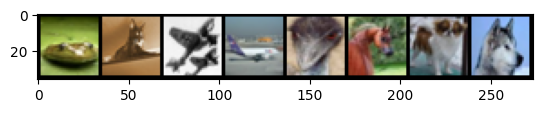
frog cat airplane airplane bird horse dog dog
10.2.3. Define a convolutional neural network
Fig. 10.4 shows a typical convolutional neural network (CNN) architecture. There are several filter kernels per convolutional layer, resulting in layers of feature maps that each receives the same input but extracts different features due to different weight matrices (to be learnt). Subsampling corresponds to pooling operations that reduces the dimensionality of the feature maps. The last layer is a fully connected layer (also called a dense layer) that performs the classification.
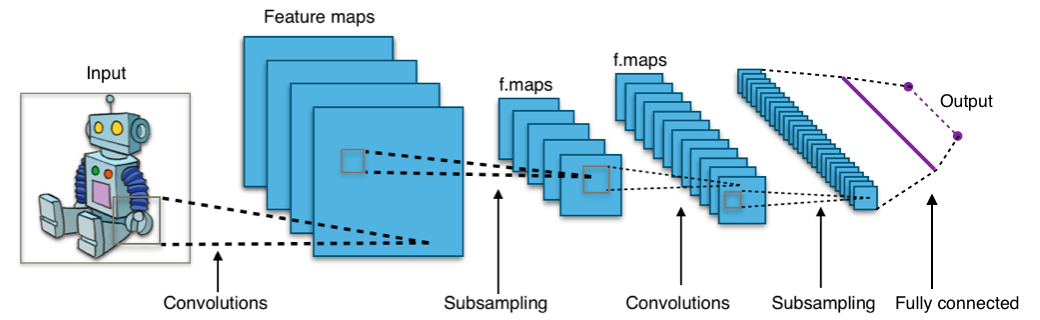
Fig. 10.4 A typical convolutional neural network (CNN) architecture.
Let us look at operations in CNNs in detail.
10.2.3.1. Convolution layer with a shared kernel/filter
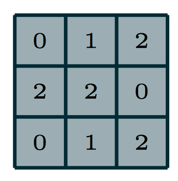
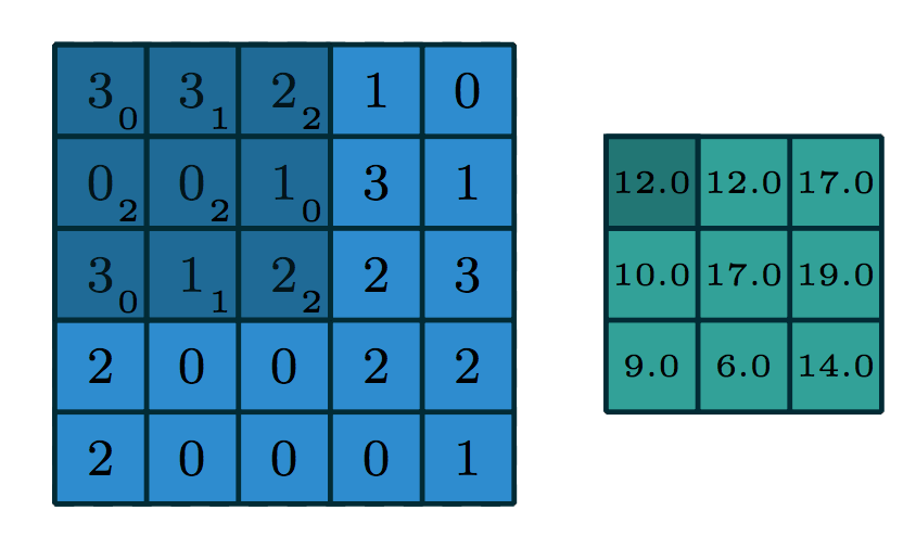
The light blue grid (middle) is the input that we are given, e.g. a 5 pixel by 5 pixel greyscale image. The grey grid (left) is a convolutional kernel/filter of size \(3 \times 3\), containing the parameters of this neural network layer.
To compute the output, we superimpose the kernel on a region of the image. Let’s start at the top left, in the dark blue region. The small numbers in the bottom right corner of each grid element corresponds to the number in the kernel. To compute the output at the corresponding location (top left), we “dot” the pixel intensities in the square region with the kernel. That is, we perform the computation:
(3 * 0 + 3 * 1 + 2 * 2) + (0 * 2 + 0 * 2 + 1 * 0) + (3 * 0 + 1 * 1 + 2 * 2)
12
The green grid (right) contains the output of this convolution layer. This output is also called an output feature map. The terms feature, and activation are interchangeable in neural networks. The output value on the top left of the green grid is consistent with the value we obtained by hand in Python.
To compute the next activation value (say, one to the right of the previous output), we will shift the superimposed kernel over by one pixel:
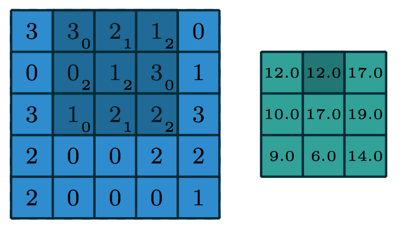
The dark blue region is moved to the right by one pixel. We again dot the pixel intensities in this region with the kernel to get another 12, and continues to get 17, \(\ldots\), 14. The green grid is updated accordingly.
Shrinked output: Here, we did not use zero padding (at the edges) so the output of this layers is shrinked by 1 on all sides. If the kernel size is \(k=2m+1\), the output will be shrinked by \(m\) on all sides so the width and height will be both reduced by \(2m\).
10.2.3.2. Convolutions with multiple input/output channels
For a colour image, the kernel will be a 3-dimensional tensor. This kernel will move through the input features just like before, and we “dot” the pixel intensities with the kernel at each region, exactly like before. This “size of the 3rd (colour) dimension” is called the number of input channels or number of input feature maps.
We also want to detect multiple features, e.g. both horizontal edges and vertical edges. We would want to learn many convolutional filters on the same input. That is, we would want to make the same computation above using different kernels, like this:
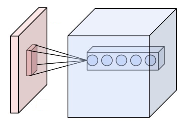
Each circle on the right of the image represents the output of a different kernel dotted with the highlighted region on the right. So, the output feature is also a 3-dimensional tensor. The size of the new dimension is called the number of output channels or number of output feature maps. In the picture above, there are 5 output channels.
The Conv2d layer expects as input a tensor in the format “NCHW”, meaning that the dimensions of the tensor should follow the order:
batch size
channel
height
width
Let us create a convolutional layer using nn.Conv2d:
myconv1 = nn.Conv2d(
    in_channels=3,  # number of input channels
    out_channels=7,  # number of output channels
    kernel_size=5,
)  # size of the kernel
Emulate a batch of 32 colour images, each of size 128x128, like the following:
x = torch.randn(32, 3, 128, 128)
y = myconv1(x)
y.shape
torch.Size([32, 7, 124, 124])
The output tensor is also in the “NCHW” format. We still have 32 images, and 7 channels (consistent with the value of out_channels of Conv2d), and of size 124x124. If we added the appropriate padding to Conv2d, namely padding = \(m\) (the kernel_size: \(2m+1\)), then our output width and height should be consistent with the input width and height.
myconv2 = nn.Conv2d(in_channels=3, out_channels=7, kernel_size=5, padding=2)

x = torch.randn(32, 3, 128, 128)
y = myconv2(x)
y.shape
torch.Size([32, 7, 128, 128])
Examine the parameters of myconv2:
conv_params = list(myconv2.parameters())
print("len(conv_params):", len(conv_params))
print("Filters:", conv_params[0].shape)  # 7 filters, each of size 3 x 5 x 5
print("Biases:", conv_params[1].shape)
len(conv_params): 2
Filters: torch.Size([7, 3, 5, 5])
Biases: torch.Size([7])
10.2.3.3. Pooling layers for subsampling
A pooling layer can be created like this:
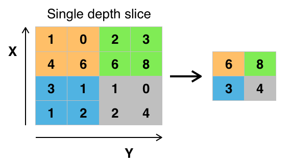
mypool = nn.MaxPool2d(kernel_size=2, stride=2)
y = myconv2(x)
z = mypool(y)
z.shape
torch.Size([32, 7, 64, 64])
Usually, the kernel size and the stride length will be equal so each pixel is pooled only once. The pooling layer has no trainable parameters:
list(mypool.parameters())
[]
10.2.3.4. Define a CNN class
Now we define a CNN class consisting of several layers as defined below (from the official the Pytorch tutorial).
class CNN(nn.Module):
    def __init__(self):
        super(CNN, self).__init__()
        self.conv1 = nn.Conv2d(
            3, 6, 5
        )  # 3=#input channels; 6=#output channels; 5=kernel size
        self.pool = nn.MaxPool2d(2, 2)
        self.conv2 = nn.Conv2d(6, 16, 5)
        self.fc1 = nn.Linear(16 * 5 * 5, 120)
        self.fc2 = nn.Linear(120, 84)
        self.fc3 = nn.Linear(84, 10)

    def forward(self, x):
        x = self.pool(F.relu(self.conv1(x)))
        x = self.pool(F.relu(self.conv2(x)))
        x = x.view(-1, 16 * 5 * 5)
        x = F.relu(self.fc1(x))
        x = F.relu(self.fc2(x))
        x = self.fc3(x)
        return x


myCNN = CNN()
Here, __init__() defines the layers. forward() defines the forward pass that transforms the input to the output. backward() is automatically defined using autograd. relu() is the rectified linear unit activation function that performs a nonlinear transformation/mapping of an input variable (element-wise operation). Conv2d() defines a convolution layer, as shown below where blue maps indicate inputs, and cyan maps indicate outputs.
Convolution with no padding, no strides.  |
More convolution layers are illustrated nicely at Convolution arithmetic (click to explore).
As defined above, this network CNN() has two convolutional layers: conv1 and conv2.
The first convolutional layer
conv1requires an input with 3 channels, outputs 6 channels, and has a kernel size of \(5\times 5\). We are not adding any zero-padding.The second convolutional layer
conv2requires an input with 6 channels (note this MUST match the output channel number of the previous layer), outputs 16 channels, and has a kernel size of (again) \(5\times 5\). We are not adding any zero-padding.
In the forward function, we see that the convolution operations are always followed by the usual ReLU activation function, and a pooling operation. The pooling operation used is max pooling, so each pooling operation
reduces the width and height of the neurons in the layer by half.
Because we are not adding any zero padding, we end up with \(16\times 5\times 5\) hidden units
after the second convolutional layer (16 matches the output channel number of conv2, \(5\times 5\) is based on the input dimension \(32\times 32\), see below). These units are then passed to two fully-connected layers, with the usual ReLU activation in between.
Notice that the number of channels grew in later convolutional layers! However, the number of hidden units in each layer is still reduced because of the convolution and pooling operation:
Initial Image Size: \(3 \times 32 \times 32 \)
After
conv1: \(6 \times 28 \times 28\) (\(32 \times 32\) is reduced by2on each side)After Pooling: \(6 \times 14 \times 14 \) (image size halved)
After
conv2: \(16 \times 10 \times 10\) (\(14 \times 14\) is reduced by2on each side)After Pooling: \(16 \times 5 \times 5 \) (halved)
After
fc1: \(120\)After
fc2: \(84\)After
fc3: \(10\) (= number of classes)
This pattern of doubling the number of channels with every pooling / strided convolution is common in modern convolutional architectures. It is used to avoid loss of too much information within a single reduction in resolution.
10.2.3.5. Inspect the CNN architecture
Now let’s take a look at the CNN built.
print(myCNN)
CNN(
  (conv1): Conv2d(3, 6, kernel_size=(5, 5), stride=(1, 1))
  (pool): MaxPool2d(kernel_size=2, stride=2, padding=0, dilation=1, ceil_mode=False)
  (conv2): Conv2d(6, 16, kernel_size=(5, 5), stride=(1, 1))
  (fc1): Linear(in_features=400, out_features=120, bias=True)
  (fc2): Linear(in_features=120, out_features=84, bias=True)
  (fc3): Linear(in_features=84, out_features=10, bias=True)
)
Let us check the (randomly initialised) parameters of this NN. Below, we check the first 2D convolution.
params = list(myCNN.parameters())
print(len(params))
print(params[0].size())  # First Conv2d's .weight
print(params[1].size())  # First Conv2d's .bias
print(params[1])
10
torch.Size([6, 3, 5, 5])
torch.Size([6])
Parameter containing:
tensor([-0.0989, -0.0496, -0.1128,  0.0413, -0.0896, -0.1129],
       requires_grad=True)
In the above, we only printed the bias values. The weight values are printed below.
print(params[0])
Parameter containing:
tensor([[[[ 0.1138,  0.0408,  0.0734,  0.0200, -0.0080],
          [ 0.0111,  0.1143,  0.0246,  0.0822,  0.0301],
          [-0.0773,  0.1006, -0.0153,  0.0356,  0.0892],
          [ 0.0176,  0.0695,  0.0711,  0.0300,  0.0492],
          [ 0.0195, -0.0609,  0.0954, -0.0673,  0.0983]],

         [[ 0.0974,  0.0102, -0.0018,  0.1078,  0.0974],
          [-0.0466, -0.0194,  0.0448, -0.0552,  0.0978],
          [ 0.0281, -0.0740, -0.0861, -0.0442, -0.1118],
          [ 0.0772, -0.0824,  0.0344,  0.1060, -0.0145],
          [-0.0125, -0.0545,  0.0635,  0.0003, -0.0113]],

         [[-0.0520, -0.0422, -0.0959, -0.0184,  0.0786],
          [-0.0044, -0.0179, -0.0160,  0.0864, -0.0296],
          [ 0.0733, -0.1011, -0.0556,  0.1047,  0.1017],
          [ 0.0272, -0.0096,  0.0345,  0.0407, -0.0175],
          [-0.0337, -0.0535,  0.0572,  0.0707,  0.0284]]],


        [[[ 0.0623,  0.0273, -0.0367,  0.0718, -0.0811],
          [-0.0275,  0.0454, -0.0328, -0.0885,  0.0423],
          [ 0.0907, -0.0959,  0.0654,  0.0857, -0.0192],
          [-0.0138, -0.0696, -0.0164, -0.0336,  0.0204],
          [-0.0788, -0.0953,  0.1080,  0.0597,  0.1106]],

         [[-0.0365, -0.1136, -0.0948,  0.1027,  0.0072],
          [-0.0707,  0.0603,  0.1098, -0.0833, -0.0753],
          [ 0.0438,  0.0462, -0.0209,  0.0827, -0.0259],
          [-0.0012, -0.0897,  0.0715, -0.0848, -0.0228],
          [ 0.0849,  0.0020,  0.0288,  0.0319, -0.0846]],

         [[ 0.0739, -0.0116,  0.0027,  0.0860,  0.1152],
          [-0.1133,  0.0306,  0.0142, -0.0993,  0.0909],
          [ 0.0487, -0.0195, -0.0420,  0.0304, -0.0968],
          [-0.0454, -0.0509,  0.0288,  0.0643, -0.0765],
          [ 0.0119, -0.0340,  0.0893, -0.0860,  0.0218]]],


        [[[ 0.0208,  0.1086,  0.0069, -0.0535, -0.1025],
          [-0.1101,  0.1003,  0.1090, -0.0028,  0.0928],
          [ 0.1042,  0.0209, -0.0525, -0.0952,  0.0765],
          [-0.0812,  0.1138,  0.0335,  0.0385,  0.1032],
          [ 0.0277,  0.0137,  0.1055, -0.1069, -0.0563]],

         [[ 0.0630,  0.0366,  0.0446,  0.0400, -0.0409],
          [ 0.0954, -0.0805, -0.0427,  0.1027,  0.0433],
          [-0.0720,  0.1148, -0.0333,  0.0179,  0.0334],
          [-0.0698,  0.1135, -0.0724, -0.0266,  0.0199],
          [ 0.0315, -0.0726, -0.0299, -0.0907, -0.1139]],

         [[ 0.0434,  0.0063, -0.0813,  0.0439,  0.0009],
          [ 0.0702,  0.0820,  0.0990,  0.0772,  0.0586],
          [ 0.0062,  0.0616,  0.0058, -0.1017, -0.0945],
          [ 0.0700,  0.0243, -0.0813, -0.1030,  0.0254],
          [ 0.0678, -0.0301, -0.0638, -0.0089, -0.0021]]],


        [[[ 0.0398,  0.0358, -0.0933, -0.0237,  0.1143],
          [ 0.1031,  0.0835,  0.0920,  0.0616, -0.0653],
          [ 0.0984,  0.0182,  0.0072,  0.0319, -0.1100],
          [ 0.0078,  0.0002,  0.0684, -0.0747, -0.0136],
          [-0.0570,  0.0959,  0.0812, -0.1117, -0.0992]],

         [[-0.0933,  0.0174, -0.0102,  0.1003, -0.0719],
          [ 0.1093,  0.0987, -0.0292, -0.0196,  0.0804],
          [-0.0928,  0.1011, -0.0114, -0.0264,  0.0993],
          [-0.0561, -0.0692,  0.0140,  0.0443,  0.0464],
          [ 0.0255,  0.0277,  0.0938,  0.0013, -0.0763]],

         [[-0.0310, -0.0790, -0.0483, -0.0298,  0.0580],
          [ 0.0951, -0.1061,  0.0407, -0.0042, -0.0967],
          [ 0.0308, -0.1023, -0.0093,  0.0749,  0.0124],
          [-0.0408, -0.0081, -0.0017,  0.0894,  0.0442],
          [-0.0949,  0.0187, -0.0939,  0.1036, -0.0496]]],


        [[[ 0.0148,  0.0268, -0.0893, -0.0045, -0.0629],
          [-0.0248, -0.1120,  0.0222, -0.0433, -0.0437],
          [ 0.0253,  0.0243, -0.0365, -0.0132,  0.1152],
          [-0.0720, -0.1113,  0.0223, -0.0117, -0.0448],
          [-0.1071,  0.0895,  0.0971,  0.0254,  0.0571]],

         [[ 0.0224,  0.0436, -0.1002,  0.0412, -0.0520],
          [-0.1036,  0.0055, -0.0654,  0.0353, -0.0587],
          [-0.0601,  0.0942,  0.0731,  0.0032,  0.0288],
          [-0.0871,  0.1138,  0.0518,  0.1023,  0.0327],
          [-0.0436, -0.0946, -0.0278,  0.0700, -0.0921]],

         [[-0.0050,  0.0009,  0.0991,  0.1073,  0.0401],
          [-0.0769, -0.1047,  0.0837,  0.0887, -0.0269],
          [-0.0571, -0.1107,  0.0756, -0.0346, -0.0020],
          [-0.0309, -0.0708, -0.0585, -0.0456,  0.0259],
          [ 0.0201,  0.1098, -0.0921, -0.0418, -0.0331]]],


        [[[ 0.0224, -0.0453, -0.0797, -0.0127,  0.0120],
          [-0.0896, -0.0800, -0.0544, -0.0020, -0.0806],
          [ 0.1094,  0.0306,  0.0580, -0.0623, -0.0548],
          [ 0.0077, -0.0655,  0.0712, -0.0851,  0.0824],
          [ 0.0527,  0.1011, -0.0267,  0.0288, -0.0267]],

         [[ 0.0133,  0.0161,  0.0996, -0.0323,  0.0088],
          [ 0.0625, -0.0158,  0.0756, -0.1089, -0.1031],
          [ 0.0447, -0.1066,  0.0304, -0.0111, -0.0194],
          [ 0.1117,  0.0202,  0.0169, -0.0088, -0.0380],
          [ 0.0206, -0.1049, -0.0802, -0.0474,  0.0173]],

         [[-0.0563, -0.0601,  0.0156,  0.0659, -0.0031],
          [-0.0747,  0.0664,  0.0448, -0.1152,  0.0046],
          [ 0.0750,  0.0587,  0.0844, -0.1062, -0.0331],
          [ 0.0087,  0.0690, -0.0112, -0.0397,  0.0041],
          [ 0.0629, -0.0020,  0.0010, -0.0983,  0.1130]]]], requires_grad=True)
To learn more about these functions, refer to the torch.nn documentation (search for the function, e.g., search for torch.nn.ReLU and you will find its documentation.
10.2.4. Optimisation, training and testing
10.2.4.1. Choose a criterion and an optimiser
Here, we choose the cross-entropy loss as the criterion and the stochastic gradient descent (SGD) with momentum as the optimiser.
criterion = nn.CrossEntropyLoss()
optimizer = optim.SGD(myCNN.parameters(), lr=0.001, momentum=0.9)
10.2.4.2. Train the network
Next, we will feed data to our CNN to train it, i.e. learn its parameters so that the criterion above (cross-entropy loss) is minimised, using the SGD optimiser. The dataset is loaded in batches to train the model. One epoch means one cycle through the full training dataset. The steps are
Define the optimisation criterion and optimisation method.
Iterate through the whole dataset in batches, for a number of
epochstill a maximum specified or a convergence criteria (e.g., successive change of loss < 0.000001)In each batch processing, we
do a forward pass
compute the loss
backpropagate the loss via
autogradupdate the parameters
Now, we loop over our data iterator, and feed the inputs to the network and optimize. Here, we set max_epochs to 3 for quick testing. In practice, more epochs typically lead to better performance.
max_epochs = 3
for epoch in range(max_epochs):  # loop over the dataset multiple times
    running_loss = 0.0
    for i, data in enumerate(train_loader, 0):
        # get the inputs; data is a list of [inputs, labels]
        inputs, labels = data

        # zero the parameter gradients
        optimizer.zero_grad()

        # forward + backward + optimize
        outputs = myCNN(inputs)
        loss = criterion(outputs, labels)
        loss.backward()
        optimizer.step()

        # print statistics
        running_loss += loss.item()
        if i % 2000 == 1999:  # print every 2000 mini-batches
            print("[%d, %5d] loss: %.3f" % (epoch + 1, i + 1, running_loss / 2000))
            running_loss = 0.0

print("Finished Training!")
[1, 2000] loss: 2.249
[1, 4000] loss: 1.866
[1, 6000] loss: 1.650
[2, 2000] loss: 1.540
[2, 4000] loss: 1.463
[2, 6000] loss: 1.402
[3, 2000] loss: 1.340
[3, 4000] loss: 1.303
[3, 6000] loss: 1.281
Finished Training!
Take a look at how autograd keeps track of the gradients for back propagation.
print(loss.grad_fn)
print(loss.grad_fn.next_functions[0][0])
<NllLossBackward0 object at 0x7fe962327910>
<LogSoftmaxBackward0 object at 0x7fe9623278b0>
10.2.4.3. Save our trained model:
PATH = root_dir + "/cifar_net.pth"
torch.save(myCNN.state_dict(), PATH)
10.2.4.4. Test the network on the test data
We will test the trained network by predicting the class label that the neural network outputs, and checking it against the ground-truth.
Firstly, let us show some images from the test set and their ground-truth labels.
dataiter = iter(test_loader)
images, labels = next(dataiter)

# print images
imshow(torchvision.utils.make_grid(images))
print(
    "GroundTruth: ",
    " ".join("%5s" % train_dataset.classes[labels[j]] for j in range(batch_size)),
)
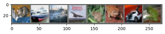
GroundTruth: cat ship ship airplane frog frog automobile frog
Next, load back in our saved model (note: saving and re-loading wasn’t necessary here, we only did it for illustration):
loadCNN = CNN()
loadCNN.load_state_dict(torch.load(PATH))
<All keys matched successfully>
Now, let us see what the neural network thinks these examples above are:
outputs = loadCNN(images)
The outputs are energies for the 10 classes. The higher the energy for a class, the more the network thinks that the image is of the particular class. Thus, let us find the index of the highest energy to get the predicted class.
_, predicted = torch.max(outputs, 1)

print(
    "Predicted: ",
    " ".join("%5s" % train_dataset.classes[predicted[j]] for j in range(batch_size)),
)
Predicted: cat ship ship airplane deer frog automobile deer
We should get at least half correct.
Let us look at how the network performs on the whole dataset.
correct = 0
total = 0
with torch.no_grad():  # testing phase, no need to compute the gradients to save time
    for data in test_loader:
        images, labels = data
        outputs = loadCNN(images)
        _, predicted = torch.max(outputs.data, 1)
        total += labels.size(0)
        correct += (predicted == labels).sum().item()

print(
    "Accuracy of the network on the 10000 test images: %d %%" % (100 * correct / total)
)
Accuracy of the network on the 10000 test images: 55 %
We should get something above 50%, which is much better than random guessing.
Let us examine what are the classes that performed well, and the classes that did not perform well:
class_correct = list(0.0 for i in range(10))
class_total = list(0.0 for i in range(10))
with torch.no_grad():
    for data in test_loader:
        images, labels = data
        outputs = loadCNN(images)
        _, predicted = torch.max(outputs, 1)
        c = (predicted == labels).squeeze()
        for i in range(batch_size):
            label = labels[i]
            class_correct[label] += c[i].item()
            class_total[label] += 1

for i in range(10):
    print(
        "Accuracy of %5s : %2d %%"
        % (train_dataset.classes[i], 100 * class_correct[i] / class_total[i])
    )
Accuracy of airplane : 59 %
Accuracy of automobile : 57 %
Accuracy of  bird : 32 %
Accuracy of   cat : 35 %
Accuracy of  deer : 51 %
Accuracy of   dog : 52 %
Accuracy of  frog : 58 %
Accuracy of horse : 67 %
Accuracy of  ship : 76 %
Accuracy of truck : 65 %
We can see that the network performs well on some classes but poorly on others, noting that we only trained it for 3 epochs.
10.2.5. Exercises
1. Suppose we have a fully connected neural network (multilayer perceptron) with \(3\) inputs and \(2\) outputs. In between, we have three hidden layers, i.e., Hidden Layer \(1\) (\(4\) neurons) after the input layer, Hidden Layer \(2\) (\(6\) neurons) after Hidden Layer \(1\), and Hidden Layer \(3\) (\(5\) neurons) after Hidden Layer \(2\), with full connections between all adjacent layers and no other connections. The activation function sigma (sigmoid) is used in the hidden layers. How many learnable parameters in total are there for this three-hidden-layer neural network?
Compare your answer with the solution below
Firstly we must count all of the weights which connect the layers of our model,
Number of weights = \((3 × 4) + (4 × 6) + (6 × 5) + (5 × 2) = 76\)
Next, we count all of the bias parameters,
Number of biases = \(4 + 6 + 5 + 2 = 17\).
The sum of these two values is the total number of model parameters, therefore the answer is \(76 + 17 = 93\).
2. We have a \(512 × 512 × 3\) colour image. We apply \(100\) \(5 × 5\) filters with stride \(7\) and pad \(2\) to obtain a convolution output. What is the output volume size? How many parameters are needed for such a layer?
Compare your answer with the solution below
Size of output:
Size of output: \((Image Length - Filter Size + 2× Padding) / Stride + 1\)
Image Length = \(512\)
Filter Size = \(5\)
Stride = \(7\)
Padding = \(2\)
After applying the first \(5 × 5\) filter:
Output Size After First Filter = \((512 − 5 + 2 × 2)/7 + 1 = 74\)
Final Output Shape = Number of Filters × Output Size × Output Size
Final Output Shape = \(100 × 74 × 74\)
Number of parameters:
Number of parameters = \((Filter Width × Filter Height × Filters in Previous Layer +1) × Number of Filters\)
Filter Width = \(5\)
Filter Height = \(5\)
Filters in Previous Layer = \(3\)
Number of Filters = \(100\)
Number of parameters = \((5 × 5 × 3 + 1) × 100 = 7600\)
3. OCTMNIST is based on an existing dataset of 109,309 valid optical coherence tomography (OCT) images for retinal diseases, with 4 different types, leading to a multi-class classification task. The source training set is split with a ratio of 9 : 1 into training and validation sets, and uses its source validation set as the test set.
Note: The paragraph above describes how the authors construct OCTMNIST from the source dataset, provided as background information. You do not have to use this information to complete the follwing exercises. OCTMNIST has fixed training, validation, and test sets with respective APIs so you just need to use the provided API and splits in OCTMNIST.
Follow the instructions at https://github.com/MedMNIST/MedMNIST to download and load the data. Use a similar method to the one you used in Exercise 1 in Section 10.1.8 to fetch the data. Again, use the torchvision package to compose a transformation to convert the data to tensors and normalise it (although this time, don’t flatten the data!). In your training, validation and testing dataloaders, use a batch size of 256.
# Install medmnist
!python -m pip install medmnist
# Write your code below to answer the question
Compare your answer with the reference solution below
# Imports
import numpy as np
import time

import torch
import torch.nn as nn
import torch.optim as optim
from torchvision import datasets, transforms
from torch.utils import data as torch_data

# For visualising data
import matplotlib.pyplot as plt
import seaborn as sns

%matplotlib inline

import medmnist

from medmnist import INFO

SEED = 1234
torch.manual_seed(SEED)
np.random.seed(SEED)

DS_INFO = INFO["octmnist"]
data_class = getattr(medmnist.dataset, DS_INFO["python_class"])

# We need to download and normalise the data. ToTensor() transforms images from 0-255 to 0-1, and Normalize() centres the data around 0, between -1 to 1.
transform = transforms.Compose(
    [
        transforms.ToTensor(),
        transforms.Normalize((0.5), (0.5)),  # Normalize the image data
    ]
)


train_dataset = data_class(split="train", download=True, transform=transform)
val_dataset = data_class(split="val", download=True, transform=transform)
test_dataset = data_class(split="test", download=True, transform=transform)

# First, lets make our data loader. We need to pick a batch size.
batch_size = 256
train_loader = torch_data.DataLoader(train_dataset, batch_size=batch_size, shuffle=True)
val_loader = torch_data.DataLoader(val_dataset, batch_size=batch_size, shuffle=True)
test_loader = torch_data.DataLoader(test_dataset, batch_size=batch_size, shuffle=True)
4. Display at least ten images for each class, i.e. at least \(40\) images, from the training set loaded in Exercise 3.
# Write your code below to answer the question
Compare your answer with the reference solution below
# Function to display the images from the dataset given a class
def display_samples(data, labels, count=10):
    """
    Display 'count' images from the dataset 'data' with label from list of labels 'labels'
    '"""

    fig, ax = plt.subplots(len(labels), count, figsize=(4 * count, 16))

    for label in labels:
        data_with_label = data.imgs[data.labels[:, 0] == label][:count]
        for ex_idx in range(len(data_with_label)):
            ax[label, ex_idx].imshow(data_with_label[ex_idx])

            # Turn off x,y ticks
            ax[label, ex_idx].set_yticks([])
            ax[label, ex_idx].set_xticks([])

        # Set the y axis label
        ax[label, 0].set_ylabel(
            ylabel=DS_INFO["label"][str(label)].split(" ")[0], fontsize=30
        )

    plt.show()


display_samples(train_dataset, [0, 1, 2, 3], 10)
5. This question asks you to design convolutional neural networks (CNNs). Only the number of convolutional (Conv) layers and the number of fully connected (FC) layers will be specified below. You are free to design other aspects of the network. For example, you can use other types of operation (e.g. padding), layers (e.g. pooling, or preprocessing (e.g. augmentation), and you will need to choose the number of units/neurons in each layer. Likewise, you may need to customise the number of epochs and many other settings according to your accessible computational power.
(a) Design a CNN with two Conv layers and two FC layers. Train the model on the training set loaded in Exercise 3, and evaluate the trained model on the test set loaded in Exercise 3 using the accuracy metric.
# Write your code below to answer the question
Compare your answer with the reference solution below
import torch.nn.functional as F

torch.manual_seed(SEED)
np.random.seed(SEED)

if torch.cuda.is_available():
    device = torch.device("cuda")
else:
    device = torch.device("cpu")


# First CNN model with 2 convolutional layer and 2 fully connected layer
class CNN_1(nn.Module):
    def __init__(self):
        super(CNN_1, self).__init__()
        self.conv1 = nn.Conv2d(1, 4, 5)  # 4X24X24
        self.pool1 = nn.MaxPool2d(2, 2)  # 4X12X12
        self.conv2 = nn.Conv2d(4, 8, 5)  # 8X8X8
        self.pool2 = nn.MaxPool2d(2, 2)  # 8X4X4

        self.fc1 = nn.Linear(8 * 4 * 4, 80)
        self.fc2 = nn.Linear(80, 4)

    def forward(self, x):
        x = self.pool1(F.relu(self.conv1(x)))  # applying pooling to 1st conv
        x = self.pool2(F.relu(self.conv2(x)))  # applying pooling to the 2nd conv
        x = x.view(-1, 8 * 4 * 4)  # connecting conv with fc
        x = F.relu(self.fc1(x))
        x = self.fc2(x)
        return F.log_softmax(x, dim=1)


model = CNN_1().to(device)
optimizer = torch.optim.SGD(model.parameters(), lr=0.01, momentum=0.5)
criterion = nn.CrossEntropyLoss()


def train(epoch):
    model.train()  # Set model to training mode

    # Loop over each batch from the training set
    for batch_idx, (data, target) in enumerate(train_loader):
        # Copy data to GPU if needed
        data = data.to(device)
        target = target.to(device)

        optimizer.zero_grad()  # Zero gradient buffers
        output = model(data)  # Pass data through the network
        loss = criterion(output, torch.max(target, 1)[1])  # Calculate loss
        loss.backward()  # Backpropagate
        optimizer.step()  # Update weights

    return print("Train Epoch: {} \tLoss: {:.6f}".format(epoch, loss.data.item()))


def test(loss_vector, accuracy_vector):
    model.eval()  # Set model to evaluation mode
    test_loss, correct, total = 0, 0, 0
    acc = []
    for data, target in test_loader:
        data = data.to(device)
        target = target.to(device)
        output = model(data)
        test_loss += criterion(output, torch.max(target, 1)[1]).data.item()

        _, preds = torch.max(output, dim=1)

        acc.append(torch.tensor(torch.sum(preds == target).item() / len(preds)))

    test_loss /= len(test_loader)
    loss_vector.append(test_loss)

    accuracy = float(sum(acc) / len(acc))
    acc.clear()

    print(
        "\nValidation set: Average loss: {:.5f}, Accuracy: ({:.2f}%)\n".format(
            test_loss, accuracy
        )
    )


epochs = 1

loss_test, acc_test = [], []
for epoch in range(1, epochs + 1):
    train(epoch)
    test(loss_test, acc_test)
Train Epoch: 1 	Loss: 0.000144

Validation set: Average loss: 0.00021, Accuracy: (62.50%)
(b) Design a CNN with three Conv layers and three FC layers. Train the model on the training set, and evaluate the trained model on the test set using the accuracy metric.
# Write your code below to answer the question
Compare your answer with the reference solution below
# Initializaing second CNN model with 3 convolutional layer and 3 FC layer
class CNN_2(nn.Module):
    def __init__(self):
        super(CNN_2, self).__init__()
        self.conv1 = nn.Conv2d(1, 4, 5)  # 4X24X24
        self.pool1 = nn.MaxPool2d(2, 2)  # 4X12X12
        self.conv2 = nn.Conv2d(
            4, 8, 3, padding=1
        )  # 8X12X12(As here we have used padding=1 we have to add +2p where p is the padding thats why the +2+1=3 minused with kernal size 3 and the dimensioms remains same 12X12)
        self.pool2 = nn.MaxPool2d(2, 2)  # 8X6X6
        self.conv3 = nn.Conv2d(8, 16, 3)  # 16X4X4
        self.pool3 = nn.MaxPool2d(2, 2)  # 16X2X2

        self.fc1 = nn.Linear(16 * 2 * 2, 120)
        self.fc2 = nn.Linear(120, 80)
        self.fc3 = nn.Linear(80, 4)

    def forward(self, x):
        x = self.pool1(F.relu(self.conv1(x)))
        x = self.pool2(F.relu(self.conv2(x)))
        x = self.pool3(F.relu(self.conv3(x)))
        x = x.view(-1, 16 * 2 * 2)
        x = F.relu(self.fc1(x))
        x = F.relu(self.fc2(x))
        x = self.fc3(x)
        output = F.log_softmax(x, dim=1)
        return output


model = CNN_2().to(device)
optimizer = torch.optim.SGD(model.parameters(), lr=0.01, momentum=0.5)
criterion = nn.CrossEntropyLoss()

epochs = 1

loss_test, acc_test = [], []
for epoch in range(1, epochs + 1):
    train(epoch)
    test(loss_test, acc_test)
Train Epoch: 1 	Loss: 0.000355

Validation set: Average loss: 0.00035, Accuracy: (62.50%)