Hypothesis testing
Contents
4.1. Hypothesis testing
Hypothesis testing has been mentioned briefly in Chapter 2 Linear regression, but it has not been explained in detail. This chapter will explain the basics of hypothesis testing and how it can be used to conduct inference.
4.1.1. Inference via hypothesis testing
Hypothesis testing is a way to make inferences about a population based on a sample (of the population). Inference is the process of using sample data to make conclusions about a population. Inference is a key part of data science because we often do not have access to the entire population of interest. Instead, we have a sample of the population. Inference allows us to make conclusions about the population based on the sample.
A statistical hypothesis test answers simple “yes-or-no” questions about data, to decide whether the data at hand sufficiently support a particular hypothesis, for example
Q1. Is the coefficient \(\beta_d\) in a linear regression of \(y\) onto \(x_1, . . . , x_D\) equal to zero?
Q2. Is there a difference in the mean blood pressure of laboratory mice in the control group and laboratory mice in the treatment group?
As a formal procedure for testing a hypothesis, the hypothesis test is based on a null hypothesis and an alternative hypothesis. The null hypothesis is a statement about the population that is assumed to be true. The alternative hypothesis is a statement about the population that is assumed to be false. The null hypothesis is often denoted by \(H_0\) and the alternative hypothesis is often denoted by \(H_1\).
Watch the 14-minute video below for a visual explanation of hypothesis testing in the context of testing drugs for treatment.
Video
Explaining Hypothesis Testing by StatQuest, embedded according to YouTube’s Terms of Service.
4.1.2. Four steps of hypothesis testing
The four steps of hypothesis testing are:
Define the null hypothesis and the alternative hypothesis.
Construct a test statistic that summarizes the strength of evidence against the null hypothesis.
Compute a \(p\)-value that quantifies the probability of having obtained a comparable or more extreme value of the test statistic under the null hypothesis.
Decide whether to reject the null hypothesis based on the \(p\)-value.
4.1.2.1. Step 1: Define the null and alternative hypotheses
In hypothesis testing, we consider two possibilities: the null hypothesis and the alternative hypothesis. The null hypothesis \(H_0\) is the default state of belief about the world. For example, the null hypotheses associated with the two questions Q1 and Q2 above are:
Q1. The coefficient \(\beta_d\) in a linear regression of \(y\) onto \(x_1, . . . , x_D\) is equal to zero.
Q2. There is no difference between the mean blood pressure of mice in the control and treatment groups.
The alternative hypothesis \(H_1\) is the opposite of the null hypothesis, representing something different and often more interesting to us, e.g., there is a difference between the mean blood pressure of the mice in the two groups.
Typically, we focus on using data to reject \(H_0\), if there is sufficient evidence in favor of \(H_1\). We can consider rejecting \(H_0\) as making a discovery about our data, i.e., we are discovering that \(H_0\) does not hold! However, if we fail to reject \(H_0\), we are not making a discovery, but we are not necessarily saying that \(H_0\) is true. We are simply saying that we do not have sufficient evidence to reject \(H_0\), since there can be multiple reasons for failing to reject \(H_0\), e.g., the null hypothesis is true, or the sample size is too small, or the test statistic is not sensitive enough to detect a difference between the two groups.
4.1.2.2. Step 2: Construct a test statistic
Next, we use our data to find evidence for or against the null hypothesis. A test statistic, often denoted by \(T\), is a function of the data that summarises the strength of evidence against the null hypothesis. Such function is often constructed from the sample mean and the sample standard deviation.
For example, denote the blood pressure measurements for the \(D_t\) mice in the treatment group as \(x^t_1, \cdots, x^t_{D_t}\) and the blood pressure measurements for the \(D_c\) mice in the control group as \(x^c_1, \cdots, x^c_{D_c}\). Denote their means as \(\mu_t\) and \(\mu_c\), respectively. Then, the test statistic for the two-sample \(t\)-test for testing \(H_0: \mu_t = \mu_c\) versus \(H_1: \mu_t \neq \mu_c\) is
where \(\hat{\mu}_t\) and \(\hat{\mu}_c\) are the sample means of the treatment and control groups, respectively, and \(s^2_t\) and \(s^2_c\) are the sample variances of the treatment and control groups, respectively.
How to interpret this statistic?
This test statistic \(T\) is a measure of the difference between the two sample means, scaled by the standard deviation of the two samples. The larger the test statistic \(T\), the more evidence there is against the null hypothesis \(H_0\) (and in support of the alternative hypothesis \(H_1\)). The smaller the test statistic \(T\), the more evidence there is in favor of the null hypothesis \(H_0\) (and against the alternative hypothesis \(H_1\)).
The one-sample \(t\)-test for testing \(H_0: \mu = \mu_0\) versus \(H_1: \mu \neq \mu_0\) is
where \(\mu_0\) is the hypothesised (population) mean, \(\hat{\mu}\) is the sample mean, and \(s\) is the sample standard deviation.
The one-sample \(t\)-test compares one sample mean to a null hypothesis value. The two-sample \(t\)-test compares two sample means to each other, i.e. considering two independent groups. The paired \(t\)-test compares two sample means to each other, but the two groups are related to each other, i.e. “paired”, e.g., the same mice before and after treatment. The paired \(t\)-test simply calculates the difference between paired groups and then performs the one-sample \(t\)-test on the differences.
4.1.2.3. Step 3: Compute a \(p\)-value
The test statistic above is typically used to compute the \(p\)-value, which is the probability of obtaining a test statistic at least as extreme as the one observed, assuming that the null hypothesis is true. The \(p\)-value is a measure of the strength of evidence against the null hypothesis. The smaller the \(p\)-value, the more evidence there is against the null hypothesis. The larger the \(p\)-value, the more evidence there is in favor of the null hypothesis.
Watch the 11-minute video below for a visual explanation of \(p\)-value in the context of testing drugs for treatment.
Video
Explanation and interpretation of \(p\)-value by StatQuest, embedded according to YouTube’s Terms of Service.
How to interpret the \(p\)-value?
The \(p\)-value is as the fraction of the time that we would expect to see such an extreme value of the test statistic if we repeated the experiment many many times, provided that the null hypothesis is true. If the \(p\)-value is small, then we would expect to see such an extreme value of the test statistic only a small fraction of the time, if we repeated the experiment many many times, provided that the null hypothesis is true. In this case, we would have strong evidence against the null hypothesis. If the \(p\)-value is large, then we would expect to see such an extreme value of the test statistic a large fraction of the time, if we repeated the experiment many many times, provided that the null hypothesis is true. In this case, we would have weak evidence against the null hypothesis.
In Step 2, we pointed out that a large (absolute) value of the test statistic provides evidence against \(H_0\). Suppose a data analyst conducts a statistical test, and reports a test statistic of \(T\) = 17.3. Does this provide strong evidence against \(H_0\)? It’s impossible to know without more information: we would need to know what value of the test statistic should be expected, under \(H_0\), if the data analyst had repeated the experiment many times. If the data analyst had repeated the experiment many times, and the test statistic was typically around 0, then a value of 17.3 would be very unusual, and we would have strong evidence against \(H_0\). However, if the data analyst had repeated the experiment many times, and the test statistic was typically around 10, then a value of 17.3 would be less unusual, and we would have weaker evidence against \(H_0\).
This is exactly what a \(p\)-value measures. A \(p\)-value allows us to transform (or standardise) our test statistic, which is measured on some arbitrary and uninterpretable scale, into a number between 0 and 1 that can be more easily interpreted.
4.1.2.4. Step 4: Decide whether to reject the null hypothesis \(H_0\)
Finally, we decide whether to reject \(H_0\) or not (we do not usually talk about “accepting” \(H_0\): instead, we talk about “failing to reject” \(H_0\)). We reject \(H_0\) if the \(p\)-value is less than a pre-specified significance level \(\alpha\). The significance level \(\alpha\) is a number between 0 and 1 that we choose before we conduct the statistical test. We typically choose \(\alpha\) = 0.05 or \(\alpha\) = 0.01, which is a common convention in the scientific community (with 0.05 being more common). If the \(p\)-value is less than \(\alpha\), then we reject \(H_0\). If the \(p\)-value is greater than or equal to \(\alpha\), then we fail to reject \(H_0\). Furthermore, a data analyst should typically report the \(p\)-value itself, rather than just whether or not it exceeds a specified threshold value.
How to interpret the significance level \(\alpha\)?
The significance level \(\alpha\) is the probability of rejecting \(H_0\) when it is true. For example, if \(\alpha\) = 0.05, then there is a 5% chance of rejecting \(H_0\) when it is true. In other words, if \(H_0\) holds, we would expect to see such a small \(p\)-value no more than 5% of the time. On the other hand, there is a 95% chance of not rejecting \(H_0\) when it is true. Nothing is absolute here.
4.1.3. Type I and Type II errors
4.1.3.1. Definition
In the context of hypothesis testing, we can distinguish between two types of errors: Type I errors and Type II errors. A Type I error occurs when we reject \(H_0\) when it is true. A Type II error occurs when we fail to reject \(H_0\) when it is false. A Type I error is also known as a false positive, and a Type II error is also known as a false negative. A summary of the possible scenarios associated with testing the null hypothesis \(H_0\) is shown in table below.
Reject \(H_0\) |
Fail to reject \(H_0\) |
|
|---|---|---|
\(H_0\) is true |
Type I error |
Correct decision |
\(H_0\) is false |
Correct decision |
Type II error |
The table above summarises the possible scenarios associated with testing the null hypothesis \(H_0\). The first row of the table shows the two possible outcomes of the statistical test (that we know after performing the test): either we reject \(H_0\) or we fail to reject \(H_0\). The first column of the table shows the two possible ground-truth values of \(H_0\) (that we do not know): either \(H_0\) is true or \(H_0\) is false. The four cells in the table show the four possible scenarios that can occur when we test \(H_0\).
If we reject \(H_0\) when it is true, then we have made a Type I error. If we fail to reject \(H_0\) when it is false, then we have made a Type II error. If we reject \(H_0\) when it is false, then we have made a correct decision. If we fail to reject \(H_0\) when it is true, then we have made a correct decision too.
The Type I error rate is defined as the probability of making a Type I error given that \(H_0\) is true, i.e., the probability of incorrectly rejecting \(H_0\). The power of the hypothesis test is defined as the probability of NOT making a Type II error given that \(H_1\) holds, i.e., the probability of correctly rejecting \(H_0\).
Connections to classification
The Type I error rate is equivalent to the false positive rate in binary classification, i.e. predicting a positive (non-null) label when the true label is in fact negative (null). The power of the hypothesis test is equivalent to the true positive rate in classification.
4.1.3.2. Trade-off between Type I and Type II errors
Ideally we would like both the Type I and Type II errors to be small. But there typically is a trade-off: we can make the Type I error small by only rejecting \(H_0\) when we have strong evidence against it, but this will increase the Type II error. We can make the Type II error small by rejecting \(H_0\) even when we have weak evidence against it, but this will increase the Type I error.
The significance level \(\alpha\) is a trade-off between the Type I and Type II errors. If we choose a small value of \(\alpha\), then we will have strong evidence against \(H_0\) when we reject it, but this will increase the Type II error. If we choose a large value of \(\alpha\), then we will have weak evidence against \(H_0\) when we reject it, but this will increase the Type I error. By only rejecting \(H_0\) when the \(p\)-value is below \(\alpha\), we ensure that the Type I error rate will be less than or equal to \(\alpha\).
In practice, we typically view Type I errors, i.e. false positives, as more “serious” than Type II errors, because the former involves declaring a scientific finding that is not correct, which is more serious than failing to declare a scientific finding (false negatives). Therefore, when we perform hypothesis testing, we typically require a low Type I error rate — e.g. at most \(\alpha\) = 0.05 — while trying to make the Type II error small (or, equivalently, the power large).
4.1.4. Hypothesis testing on synthetic data
Let us perform some one-sample \(t\)-tests on synthetic data for this study.
Get ready by importing the APIs needed from respective libraries.
import pandas as pd
import numpy as np
import matplotlib.pyplot as plt
import seaborn as sns
from scipy import stats as st
from sklearn.metrics import confusion_matrix
from statsmodels.sandbox.stats.multicomp import multipletests

%matplotlib inline
Set a random seed for reproducibility (more on this later in the next section).
np.random.seed(2022)
Let us create 100 variables, each with 10 observations (samples). We make the first 50 variables to have mean 0.5 (the offset) and variance 1, and the last 50 variables to have mean 0 and variance 1.
X = np.random.normal(loc=0.0, scale=1.0, size=(10, 100))
offset = 0.5
X[:, :50] = X[:, :50] + offset
We then perform one-sample \(t\)-tests of the null hypothesis that the population mean (popmean) is zero \(H_0: \mu_i = 0\) for all variables \(i=1, \cdots, 100\) using the ttest_1samp function from the scipy.stats module. The function returns the \(t\)-statistic and the \(p\)-value for each variable.
results = st.ttest_1samp(a=X, popmean=0)
Let us inspect the \(t\)-statistic and \(p\)-value for the first and the 60th variables.
print("Variable 0 t-statistic: ", results.statistic[0])
print("Variable 0 p-value: ", results.pvalue[0])
print("Variable 59 t-statistic: ", results.statistic[59])
print("Variable 59 p-value: ", results.pvalue[59])
Variable 0 t-statistic:  1.2087075209473424
Variable 0 p-value:  0.2575718703150701
Variable 59 t-statistic:  -0.0037602605936159984
Variable 59 p-value:  0.9970817828876111
The \(p\)-value for the first variable is 0.25, which is greater than the significance level \(\alpha\) = 0.05. Therefore, we fail to reject the null hypothesis \(H_0\) for the first variable. We know the true mean of the first variable is 0.5, so the null hypothesis is false. Thus, this is a Type II error.
The \(p\)-value for the 60th variable is 0.99. We also fail to reject the null hypothesis \(H_0\). However, we know the true mean of the 60th variable is 0, so the null hypothesis is true. Thus, this is a correct decision.
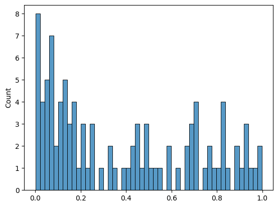
We can plot the \(p\)-values of the \(t\)-tests as a histogram to see the distribution of the \(p\)-values.
sns.histplot(results.pvalue, bins=50)
<Axes: ylabel='Count'>
We set the significance level \(\alpha\) to 0.05 to make a decision on whether to reject \(H_0\) or not.
p_values = results.pvalue
decisions = []
for i in range(len(p_values)):
    if p_values[i] < 0.05:
        decisions.append("Reject H0")
    else:
        decisions.append("Fail to reject H0")
Let us use the ground truth to evaluate the performance.
ground_truth = np.repeat(["Reject H0", "Fail to reject H0"], [50, 50], axis=0)
labels = ["Reject H0", "Fail to reject H0"]
cm = confusion_matrix(ground_truth, decisions, labels=labels)
print(cm)
[[14 36]
 [ 1 49]]
We can visualise this confusion matrix using the heatmap function from the seaborn module.
ground_truth_labels = ["H0 is False", "H0 is True"]
sns.heatmap(
    cm, annot=True, fmt="d", xticklabels=labels, yticklabels=ground_truth_labels
)
<Axes: >
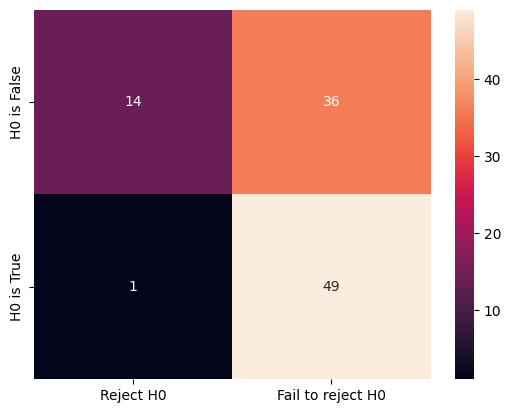
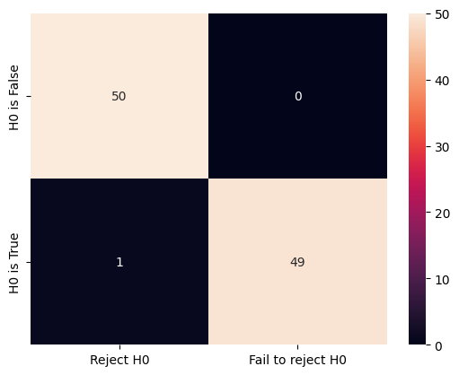
There are quite some errors made. We can make the offset larger (from 0.5 to 1) to see the change to the confusion matrix and the total number of errors.
offset = 1
decisions = []
X[:, :50] = X[:, :50] + offset
results = st.ttest_1samp(a=X, popmean=0)
p_values = results.pvalue
for i in range(len(p_values)):
    if p_values[i] < 0.05:
        decisions.append("Reject H0")
    else:
        decisions.append("Fail to reject H0")
cm = confusion_matrix(ground_truth, decisions, labels=labels)
sns.heatmap(
    cm, annot=True, fmt="d", xticklabels=labels, yticklabels=ground_truth_labels
)
<Axes: >
len(decisions)
100
For this time, there is only one error in total.
4.1.5. Multiple hypothesis testing
Let us consider the more complicated case where we wish to test \(M\) null hypotheses, \(H_0^1, H_0^2, \ldots, H_0^M\).
4.1.5.1. Case study: a “sure-win” stockbroker?
A stockbroker wishes to drum up new clients by convincing them of his/her trading acumen. S/he tells 1,024 (i.e. \(2^{10}\)) potential new clients that s/he can correctly predict whether Apple’s stock price will increase or decrease for 10 days running. For such a binary outcome, we have \(2^{10}=1024\) possibilities for the course of these 10 days. Therefore, s/he emails each client one of these 1024 possibilities. Although the vast majority of his/her potential clients will find that his/her predictions are no better than chance, one of his/her potential clients will be really impressed to find that his/her predictions were correct for ALL 10 of the days! And so the stockbroker gains a new client (and possible more when this client spreads the news).
This is part of the reason why we receive so many spam emails/calls. If you make a lot of guesses (“predictions”), then you are bound to get some right by chance.
4.1.5.2. The challenge of multiple hypothesis testing
Likewise, if we flip 1,024 fair coins ten times each. Then we would expect (on average) one coin to come up all tails. If one of our coins comes up all tails, then we might therefore conclude that this particular coin is not fair. But it would be incorrect to conclude that the coin is not fair: in fact, the null hypothesis holds, and we just happen to have gotten ten tails in a row by chance.
The examples above demonstrate the main challenge of multiple testing: when testing a huge number of null hypotheses, we are bound to get some very small \(p\)-values by chance. If we make a decision about whether to reject each null hypothesis without accounting for the fact that we have performed a very large number of tests, then we may end up rejecting a great number of true null hypotheses, i.e. making a large number of Type I errors (false positives), which is what we hope to avoid (see the above).
Why repeat the experiment?
The reason why we repeat the experiment is to reduce the chance of getting a false positive. If we only perform the experiment once, then we will have a very small chance of getting a false positive.
4.1.5.3. Family-wise error rate (FWER)
Rejecting a null hypothesis if the \(p\)-value is below \(\alpha\) controls the probability of falsely rejecting that null hypothesis at level \(\alpha\). However, if we do this for \(M\) null hypotheses, then the chance of falsely rejecting at least one of the M null hypotheses is quite a bit higher! This is because the chance of getting a false positive for each null hypothesis is \(\alpha\), but the chance of getting a false positive for at least one of the \(M\) null hypotheses is \(1-(1-\alpha)^M\).
Let us see this visually. We will plot the chance of getting a false positive for at least one of the \(M\) null hypotheses as a function of \(\alpha\) and \(M\).
m = range(500)
fwe1 = list(map(lambda x: 1 - pow(1 - 0.05, x), m))
fwe2 = list(map(lambda x: 1 - pow(1 - 0.01, x), m))
fwe3 = list(map(lambda x: 1 - pow(1 - 0.001, x), m))

plt.plot(m, fwe1, label="alpha=0.05")
plt.plot(m, fwe2, label="alpha=0.01")
plt.plot(m, fwe3, label="alpha=0.001")
plt.xlabel("M: Number of tests in log scale")
plt.ylabel("Family-wise error rate")
plt.xscale("log")
plt.legend()
plt.show()
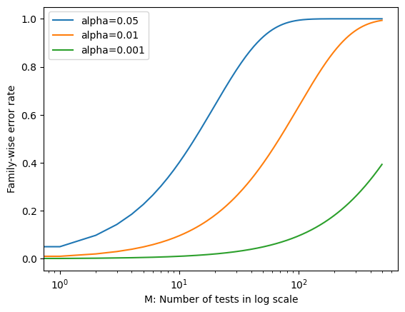
We see that setting \(\alpha = 0.05\) results in a high FWER even for moderate \(M\). With \(\alpha = 0.01\), we can test no more than five null hypotheses before the FWER exceeds 0.05. Only for very small values, such as \(\alpha = 0.001\), we can manage to ensure a small FWER for moderate values of \(M\).
Of course, the problem with setting \(\alpha\) to such a low value is that we are likely to make a large number of Type II errors: in other words, our power is very low.
To address this challenge of multiple testing, we hope to test multiple hypotheses while controlling the probability of making at least one Type I error. This can be achieved by controlling the family-wise error rate (FWER), which is the probability of making at least one Type I error when testing \(M\) null hypotheses, i.e. rejecting at least one null hypothesis when all \(M\) null hypotheses are true. The FWER is also known as the probability of a false discovery.
One solution is to adjust the significance level \(\alpha\) for each null hypothesis. The Bonferroni correction is a simple way to adjust the significance level \(\alpha\) for multiple testing. This method divides the significance level \(\alpha\) by the number of null hypotheses \(M\) to obtain the family-wise significance level \(\alpha_M\). The Bonferroni correction is conservative, i.e. it ensures that the FWER is at most \(\alpha_M\). However, it also reduces the power of the test, i.e. the chance of rejecting a false null hypothesis.
Let us study the family-wise error rate (FWER) and Bonferroni correction on the Fund dataset (click to explore).
Load the data first and display some essential information first.
fund_url = "https://github.com/pykale/transparentML/raw/main/data/Fund.csv"

fund_df = pd.read_csv(fund_url, na_values="?").dropna()
fund_df.info()
<class 'pandas.core.frame.DataFrame'>
RangeIndex: 50 entries, 0 to 49
Columns: 2000 entries, Manager1 to Manager2000
dtypes: float64(2000)
memory usage: 781.4 KB
Inspect the first few rows of the data, as usual.
fund_df.head()
| Manager1 | Manager2 | Manager3 | Manager4 | Manager5 | Manager6 | Manager7 | Manager8 | Manager9 | Manager10 | ... | Manager1991 | Manager1992 | Manager1993 | Manager1994 | Manager1995 | Manager1996 | Manager1997 | Manager1998 | Manager1999 | Manager2000 | |
|---|---|---|---|---|---|---|---|---|---|---|---|---|---|---|---|---|---|---|---|---|---|
| 0 | -3.341992 | -4.167469 | 9.389223 | 8.417220 | 0.997863 | 7.191473 | -10.767592 | 4.072425 | 1.575264 | -0.798505 | ... | -2.948706 | 10.350706 | -2.855337 | -4.431786 | 0.739544 | 0.198044 | 1.752188 | -1.534710 | -3.359419 | 6.585654 |
| 1 | 3.759627 | 12.525254 | 3.403366 | 0.143944 | -7.222227 | 0.067747 | -10.737053 | -1.138185 | -7.166604 | 4.778522 | ... | 24.003150 | -1.966606 | -1.609109 | 1.405325 | 4.717175 | 1.540359 | -12.218233 | -0.073008 | -8.547683 | -2.382629 |
| 2 | 12.970091 | -2.581061 | -0.824734 | 6.584604 | 17.050241 | 1.857130 | 3.196942 | -7.981362 | -1.214148 | 2.338250 | ... | -2.926914 | 6.420147 | 8.946921 | 3.449013 | 1.009957 | 1.481369 | 14.203314 | 0.005562 | -5.105035 | 2.292429 |
| 3 | -4.874630 | 7.981743 | -4.026743 | -4.731946 | 0.503276 | 0.740187 | -28.969410 | 4.683751 | -0.568840 | -4.000547 | ... | -3.112208 | 3.173581 | -6.017109 | -1.984873 | 1.022525 | -2.261927 | 19.345970 | -1.048299 | -0.016154 | 1.196832 |
| 4 | 2.019279 | -5.370236 | -4.854669 | 10.594432 | -6.891574 | 9.877838 | 1.430033 | 9.840311 | 5.311455 | 18.365094 | ... | 7.173653 | -9.157211 | 7.643125 | -1.022339 | -1.325865 | 2.848785 | -6.642081 | 2.488612 | 0.032060 | -7.510032 |
5 rows × 2000 columns
Let us do a one-sample \(t\)-test for the first manager.
result = st.ttest_1samp(a=fund_df["Manager1"], popmean=0)
print(result.pvalue)
0.0062023554855382655
Let’s do a one-sample \(t\)-test for five managers instead.
p_values = []
manager_number = 5

for i in range(manager_number):
    result = st.ttest_1samp(a=fund_df.iloc[:, i], popmean=0)
    p_values.append(result.pvalue)

print(p_values)
[0.0062023554855382655, 0.9182711516514124, 0.011600982682500436, 0.6005396008061651, 0.7557815084668166]
The \(p\)-values are low for Managers One and Three, and high for the other three managers. However, we cannot simply reject \(H_0^1\) and \(H_0^3\), since this would fail to account for the multiple testing that we have performed. Instead, we can use the Bonferroni correction to adjust the significance level \(\alpha\) for multiple testing, using the multipletests function from the statsmodels module.
reject, p_values_corrected, alphacSidak, alphacBonf = multipletests(
    p_values, method="bonferroni"
)
print(p_values_corrected)
[0.03101178 1. 0.05800491 1. 1. ]
Therefore, using the Bonferroni correction, we will reject the null hypothesis only for Manager One while controlling the FWER at 0.05. This information is also available in the variable reject.
print(reject)
[ True False False False False]
It is reasonable to control the FWER when \(M\) takes on a small value, like 5 or 10. However, for \(M\) = 100 or 1,000, attempting to control the FWER will make it almost impossible to reject any of the false null hypotheses.
4.1.5.4. False discovery rate
In practice, when \(M\) is large, trying to prevent any false positives (as in FWER control) is simply too stringent and scientifically uninteresting. In this case, we can tolerate a few false positives, in the interest of making more discoveries, i.e. more rejections of the null hypothesis. Thus, we typically control the false discovery rate (FDR), which is the expected proportion of rejected null hypotheses that are false. The FDR is also known as the expected proportion of false discoveries.
The Benjamini-Hochberg procedure is a popular method for controlling the FDR. This method controls the FDR at level \(\alpha\) by rejecting the null hypothesis for the \(k\)th smallest \(p\)-value if \(p_k \leq \alpha k/M\), where \(M\) is the number of null hypotheses. The Benjamini-Hochberg procedure is less conservative than the Bonferroni correction, i.e. it allows for more false positives. However, it also increases the power of the test, i.e. the chance of rejecting a false null hypothesis.
The FDR is typically more useful than the FWER when \(M\) is large. The use of the FDR also aligns well with the way that data are often collected in contemporary applications, e.g. in exploratory data analysis and genomics.
Let us study the false discovery rate (FDR) on the Fund dataset above.
p_values = []
manager_number = fund_df.shape[1]

for i in range(manager_number):
    result = st.ttest_1samp(a=fund_df.iloc[:, i], popmean=0)
    p_values.append(result.pvalue)

print(p_values[0:10])
[0.0062023554855382655, 0.9182711516514124, 0.011600982682500436, 0.6005396008061651, 0.7557815084668166, 0.0009645725984591884, 0.004651524304645157, 0.0013978025258984373, 0.002604065138148157, 0.0027967384364455815]
There are far too many managers to consider if we try to control the FWER. Instead, we focus on controlling the FDR: that is, the expected fraction of rejected null hypotheses that are actually false positives. We can use the same multipletests function from the statsmodels module to control the FDR.
reject, p_values_corrected, alphacSidak, alphacBonf = multipletests(
    p_values, method="fdr_bh"
)
print(p_values_corrected[0:10])
[0.08988921 0.991491   0.12211561 0.92342997 0.95603587 0.07513802
 0.0767015  0.07513802 0.07513802 0.07513802]
The \(p\)-values output by the Benjamini-Hochberg procedure can be interpreted as the smallest FDR threshold at which we would reject a particular null hypothesis. For instance, a \(p\)-value of 0.1 indicates that we can reject the corresponding null hypothesis at an FDR of 10% or greater, but that we cannot reject the null hypothesis at an FDR below 10%.
We would find that 146 of the 2,000 fund managers have a corrected \(p\)-value below 0.1.
sum(p_values_corrected <= 0.1)
146
If we use bonferroni method, we will find None.
sum(np.array(p_values) <= 0.1 / fund_df.shape[1])
0
Unlike \(p\)-values, the choice of FDR threshold is typically context-dependent (e.g. cost/budget-dependent), or even dataset-dependent, with no standard accepted threshold.
4.1.6. Exercises
1. The alternative hypothesis is a statement about the population that is assumed to be true.
   a. True

   b. False
Compare your answer with the solution below
b. False. The null hypothesis is assumed to be true, and we are carrying out the experiment to see if we can reject the null hypothesis in favour of the alternative hypothesis.
2. The larger the \(p\)-value, the more evidence there is in favor of the null hypothesis.
   a. True

   b. False
Compare your answer with the solution below
a. True
3. A test statistic allows us to standardise our \(p\)-value.
   a. True

   b. False
Compare your answer with the solution below
b. False. A \(p\)-value allows us to transform (or standardise) our test statistic, which is measured on some arbitrary and uninterpretable scale, into a number between 0 and 1 that can be more easily interpreted.
4. A Type II error occurs when we fail to reject \(H_0\) when it is false.
   a. True

   b. False
Compare your answer with the solution below
a. True
5. When we perform hypothesis testing, we typically require a low Type II error rate while trying to make the Type I error small.
   a. True

   b. False
Compare your answer with the solution below
b. False. We require high Type II error to make the Type I error small
6. All the following exercises involve the use of the Weekly dataset.
a. Load the dataset and inspect the first few rows of the data.
# Write your code below to answer the question
Compare your answer with the reference solution below
import pandas as pd

data_url = "https://github.com/pykale/transparentML/raw/main/data/Weekly.csv"
df = pd.read_csv(data_url)
df.head()
| Year | Lag1 | Lag2 | Lag3 | Lag4 | Lag5 | Volume | Today | Direction | |
|---|---|---|---|---|---|---|---|---|---|
| 0 | 1990 | 0.816 | 1.572 | -3.936 | -0.229 | -3.484 | 0.154976 | -0.270 | Down |
| 1 | 1990 | -0.270 | 0.816 | 1.572 | -3.936 | -0.229 | 0.148574 | -2.576 | Down |
| 2 | 1990 | -2.576 | -0.270 | 0.816 | 1.572 | -3.936 | 0.159837 | 3.514 | Up |
| 3 | 1990 | 3.514 | -2.576 | -0.270 | 0.816 | 1.572 | 0.161630 | 0.712 | Up |
| 4 | 1990 | 0.712 | 3.514 | -2.576 | -0.270 | 0.816 | 0.153728 | 1.178 | Up |
b. Perform a one-sample \(t\)-tests of the null hypothesis that the population mean (popmean) is \(0.05\), \(H_0: \mu_i = 0.5\) for variable Today from the Weekly dataset using the ttest_1samp function from the scipy.stats module and find out the \(t\)-statistic and \(p\)-value for the variable Today and state whether we can reject the null hypothesis for this variable. The \(t\)-test is calculated for the mean of one set of values. The null hypothesis is that the expected mean of a sample of independent observations is equal to the specified population mean, popmean = \(0.5\). Hint: See section 4.1.4
# Write your code below to answer the question
Compare your answer with the reference solution below
from scipy import stats as st

results = st.ttest_1samp(a=df["Today"], popmean=0.5)
print("Variable Volume t-statistic: ", results.statistic)
print("Variable Volume p-value: ", results.pvalue)

# The p-value for the Today variable is 1.09e-06, which is smaller than the significance level alpha= 0.05.
# Therefore, we can reject the null hypothesis and accept the alternative hypothesis for the Today variable.
Variable Volume t-statistic:  -4.901862226324721
Variable Volume p-value:  1.0936150729006281e-06
c. Now, do another one-sample \(t\)-test of the null hypothesis that the population mean (popmean) is \(0.05\), \(H_0: \mu_i = 0.5\) for all the lagging indicator variables (Lag1, Lag2, Lag3, Lag4, Lag5) from the Weekly dataset and show all the \(p\)-values. Hint: See section 4.1.5
# Write your code below to answer the question
Compare your answer with the reference solution below
p_values = []
lag_number = 6

for i in range(1, lag_number):
    result = st.ttest_1samp(a=df["Lag" + str(i)], popmean=0.5)
    p_values.append(result.pvalue)
print(p_values)
[1.1481677562182723e-06, 1.1912787173817803e-06, 9.402873213740145e-07, 8.511375882119721e-07, 5.656565652311808e-07]
d. According to the resulting \(p\)-values from Exercise 6(c), can we reject all the null hypotheses as the \(p\)-values are low?
Compare your answer with the solution below
The \(p\)-values are low for all the lagging indicators. However, we cannot simply reject \(H_{0}^{1}\), \(H_{0}^{2}\), \(H_{0}^{3}\), \(H_{0}^{4}\)and \(H_{0}^{5}\), since this would fail to account for the multiple testing that we have performed.
e. Now, use the Bonferroni correction to adjust the significance level \(\alpha\) for multiple testing performed in Exercise 6(c) using the multipletests function from the statsmodels module and state which null hypothesis we can reject. Hint: See section 4.1.5.2.
# Write your code below to answer the question
Compare your answer with the reference solution below
from statsmodels.sandbox.stats.multicomp import multipletests

reject, p_values_corrected, alphacSidak, alphacBonf = multipletests(
    p_values, method="bonferroni"
)
print(p_values_corrected)
print(reject)

# Therefore, using the Bonferroni correction, we will reject all the null hypothesis while controlling the FWER at 0.05.
[5.74083878e-06 5.95639359e-06 4.70143661e-06 4.25568794e-06
 2.82828283e-06]
[ True  True  True  True  True]
f. If we want to test \(100\) null hypotheses, can we control FWER using Bonferroni correction?
Compare your answer with the solution below
It is reasonable to control the FWER when \(M\) (number of the null hypothesis) takes on a small value, like \(5\) or \(10\). However, for \(M= 100\) or \(1,000\), attempting to control the FWER will make it almost impossible to reject any of the false null hypotheses. In that case, we control the false discovery rate (FDR) using the Benjamini-Hochberg procedure rather than the FWER.