Loading Data
Contents
Loading Data
Read then Launch
This content is best viewed in html because jupyter notebook cannot display some content (e.g. figures, equations) properly. You should finish reading this page first and then launch it as an interactive notebook in Google Colab (faster, Google account needed) or Binder by clicking the rocket symbol () at the top.
Data frame and basic operations
In Python, Pandas is a commonly used library to read data from files into data frames. Use the Auto.csv file (click to open) as an example. First, take a look at the csv file. There are headers, missing values are marked by ‘?’. The data is separated by comma. We can use the read_csv function to read the csv file into a data frame. The read_csv function has many parameters, we can use ? to get the documentation of the function.
The following code loads libraries needed for this section and shows how to read the csv file Auto.csv in the textbook into a data frame auto_df.
import pandas as pd
import urllib
from matplotlib import pyplot as plt

%matplotlib inline
data_url = "https://github.com/pykale/transparentML/raw/main/data/Auto.csv"
auto_df = pd.read_csv(data_url, header=0, na_values="?")
The .head() method can be used to get the first 5 (by default) rows of the data frame.
auto_df.head()
| mpg | cylinders | displacement | horsepower | weight | acceleration | year | origin | name | |
|---|---|---|---|---|---|---|---|---|---|
| 0 | 18.0 | 8 | 307.0 | 130.0 | 3504 | 12.0 | 70 | 1 | chevrolet chevelle malibu |
| 1 | 15.0 | 8 | 350.0 | 165.0 | 3693 | 11.5 | 70 | 1 | buick skylark 320 |
| 2 | 18.0 | 8 | 318.0 | 150.0 | 3436 | 11.0 | 70 | 1 | plymouth satellite |
| 3 | 16.0 | 8 | 304.0 | 150.0 | 3433 | 12.0 | 70 | 1 | amc rebel sst |
| 4 | 17.0 | 8 | 302.0 | 140.0 | 3449 | 10.5 | 70 | 1 | ford torino |
The .describe() method can get the summary statistics of the data frame. Specify the argument include to get the summary statistics of certain variables, e.g. include = "all" for mixed types, include = [np.number] for numerical columns, and include = ["O"] for objects.
auto_df.describe()
| mpg | cylinders | displacement | horsepower | weight | acceleration | year | origin | |
|---|---|---|---|---|---|---|---|---|
| count | 397.000000 | 397.000000 | 397.000000 | 392.000000 | 397.000000 | 397.000000 | 397.000000 | 397.000000 |
| mean | 23.515869 | 5.458438 | 193.532746 | 104.469388 | 2970.261965 | 15.555668 | 75.994962 | 1.574307 |
| std | 7.825804 | 1.701577 | 104.379583 | 38.491160 | 847.904119 | 2.749995 | 3.690005 | 0.802549 |
| min | 9.000000 | 3.000000 | 68.000000 | 46.000000 | 1613.000000 | 8.000000 | 70.000000 | 1.000000 |
| 25% | 17.500000 | 4.000000 | 104.000000 | 75.000000 | 2223.000000 | 13.800000 | 73.000000 | 1.000000 |
| 50% | 23.000000 | 4.000000 | 146.000000 | 93.500000 | 2800.000000 | 15.500000 | 76.000000 | 1.000000 |
| 75% | 29.000000 | 8.000000 | 262.000000 | 126.000000 | 3609.000000 | 17.100000 | 79.000000 | 2.000000 |
| max | 46.600000 | 8.000000 | 455.000000 | 230.000000 | 5140.000000 | 24.800000 | 82.000000 | 3.000000 |
auto_df.describe(include="all")
| mpg | cylinders | displacement | horsepower | weight | acceleration | year | origin | name | |
|---|---|---|---|---|---|---|---|---|---|
| count | 397.000000 | 397.000000 | 397.000000 | 392.000000 | 397.000000 | 397.000000 | 397.000000 | 397.000000 | 397 |
| unique | NaN | NaN | NaN | NaN | NaN | NaN | NaN | NaN | 304 |
| top | NaN | NaN | NaN | NaN | NaN | NaN | NaN | NaN | ford pinto |
| freq | NaN | NaN | NaN | NaN | NaN | NaN | NaN | NaN | 6 |
| mean | 23.515869 | 5.458438 | 193.532746 | 104.469388 | 2970.261965 | 15.555668 | 75.994962 | 1.574307 | NaN |
| std | 7.825804 | 1.701577 | 104.379583 | 38.491160 | 847.904119 | 2.749995 | 3.690005 | 0.802549 | NaN |
| min | 9.000000 | 3.000000 | 68.000000 | 46.000000 | 1613.000000 | 8.000000 | 70.000000 | 1.000000 | NaN |
| 25% | 17.500000 | 4.000000 | 104.000000 | 75.000000 | 2223.000000 | 13.800000 | 73.000000 | 1.000000 | NaN |
| 50% | 23.000000 | 4.000000 | 146.000000 | 93.500000 | 2800.000000 | 15.500000 | 76.000000 | 1.000000 | NaN |
| 75% | 29.000000 | 8.000000 | 262.000000 | 126.000000 | 3609.000000 | 17.100000 | 79.000000 | 2.000000 | NaN |
| max | 46.600000 | 8.000000 | 455.000000 | 230.000000 | 5140.000000 | 24.800000 | 82.000000 | 3.000000 | NaN |
The dimension of a data frame can be found out by the same .shape() method as in numpy arrays.
auto_df.shape
(397, 9)
Indexing in Pandas data frame is similar to indexing in numpy arrays. A row, a column, or a submatrix can be accessed by the .iloc[] or .loc[] method. iloc is used to index by position, and loc is used to index by labels (row and column names).
auto_df.iloc[:4, :2]
| mpg | cylinders | |
|---|---|---|
| 0 | 18.0 | 8 |
| 1 | 15.0 | 8 |
| 2 | 18.0 | 8 |
| 3 | 16.0 | 8 |
auto_df.loc[[0, 1, 2, 3], ["mpg", "cylinders"]]
| mpg | cylinders | |
|---|---|---|
| 0 | 18.0 | 8 |
| 1 | 15.0 | 8 |
| 2 | 18.0 | 8 |
| 3 | 16.0 | 8 |
There is an alternative way to select the first 4 rows.
auto_df[:4]
| mpg | cylinders | displacement | horsepower | weight | acceleration | year | origin | name | |
|---|---|---|---|---|---|---|---|---|---|
| 0 | 18.0 | 8 | 307.0 | 130.0 | 3504 | 12.0 | 70 | 1 | chevrolet chevelle malibu |
| 1 | 15.0 | 8 | 350.0 | 165.0 | 3693 | 11.5 | 70 | 1 | buick skylark 320 |
| 2 | 18.0 | 8 | 318.0 | 150.0 | 3436 | 11.0 | 70 | 1 | plymouth satellite |
| 3 | 16.0 | 8 | 304.0 | 150.0 | 3433 | 12.0 | 70 | 1 | amc rebel sst |
The column names can be found out by the list function or the .columns attribute.
print(list(auto_df))
print(auto_df.columns)
['mpg', 'cylinders', 'displacement', 'horsepower', 'weight', 'acceleration', 'year', 'origin', 'name']
Index(['mpg', 'cylinders', 'displacement', 'horsepower', 'weight',
       'acceleration', 'year', 'origin', 'name'],
      dtype='object')
.isnull() and .sum() methods can be used to find out how many NaNs in each variables.
auto_df.isnull().sum()
mpg             0
cylinders       0
displacement    0
horsepower      5
weight          0
acceleration    0
year            0
origin          0
name            0
dtype: int64
# after the previous steps, there are 397 obs in the data and only 5 with missing values. We can just drop the ones with missing values
print(auto_df.shape)
auto_df = auto_df.dropna()
print(auto_df.shape)
(397, 9)
(392, 9)
The type of variable(s) can be changed. The following example will change the cylinders into categorical variable
auto_df["cylinders"] = auto_df["cylinders"].astype("category")
Visualising data
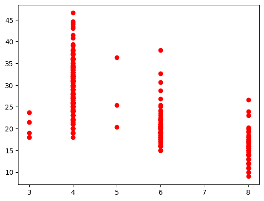
Refer to a column of data frame by name using .column_name. See the options in plt.plot for more.
plt.plot(auto_df.cylinders, auto_df.mpg, "ro")
plt.show()
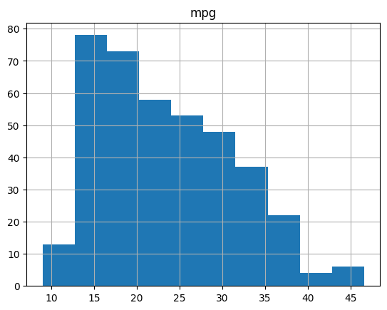
The .hist() method can get the histogram of certain variables. Specify the argument column to get the histogram of a certain variable.
auto_df.hist(column=["cylinders", "mpg"])
plt.show()
Exercises
1. This exercise is related to the College dataset. It contains a number of features for \(777\) different universities and colleges in the US.
a. Use the read_csv() function to read the data and print the first \(20\) rows of the loaded data. Make sure that you have the directory set to the correct location for the data.
# Write your code below to answer the question
Compare your answer with the reference solution below
import pandas as pd

data_url = "https://github.com/pykale/transparentML/raw/main/data/College.csv"
college_df = pd.read_csv(data_url, header=0)
college_df.head(20)
| Private | Apps | Accept | Enroll | Top10perc | Top25perc | F.Undergrad | P.Undergrad | Outstate | Room.Board | Books | Personal | PhD | Terminal | S.F.Ratio | perc.alumni | Expend | Grad.Rate | |
|---|---|---|---|---|---|---|---|---|---|---|---|---|---|---|---|---|---|---|
| 0 | Yes | 1660 | 1232 | 721 | 23 | 52 | 2885 | 537 | 7440 | 3300 | 450 | 2200 | 70 | 78 | 18.1 | 12 | 7041 | 60 |
| 1 | Yes | 2186 | 1924 | 512 | 16 | 29 | 2683 | 1227 | 12280 | 6450 | 750 | 1500 | 29 | 30 | 12.2 | 16 | 10527 | 56 |
| 2 | Yes | 1428 | 1097 | 336 | 22 | 50 | 1036 | 99 | 11250 | 3750 | 400 | 1165 | 53 | 66 | 12.9 | 30 | 8735 | 54 |
| 3 | Yes | 417 | 349 | 137 | 60 | 89 | 510 | 63 | 12960 | 5450 | 450 | 875 | 92 | 97 | 7.7 | 37 | 19016 | 59 |
| 4 | Yes | 193 | 146 | 55 | 16 | 44 | 249 | 869 | 7560 | 4120 | 800 | 1500 | 76 | 72 | 11.9 | 2 | 10922 | 15 |
| 5 | Yes | 587 | 479 | 158 | 38 | 62 | 678 | 41 | 13500 | 3335 | 500 | 675 | 67 | 73 | 9.4 | 11 | 9727 | 55 |
| 6 | Yes | 353 | 340 | 103 | 17 | 45 | 416 | 230 | 13290 | 5720 | 500 | 1500 | 90 | 93 | 11.5 | 26 | 8861 | 63 |
| 7 | Yes | 1899 | 1720 | 489 | 37 | 68 | 1594 | 32 | 13868 | 4826 | 450 | 850 | 89 | 100 | 13.7 | 37 | 11487 | 73 |
| 8 | Yes | 1038 | 839 | 227 | 30 | 63 | 973 | 306 | 15595 | 4400 | 300 | 500 | 79 | 84 | 11.3 | 23 | 11644 | 80 |
| 9 | Yes | 582 | 498 | 172 | 21 | 44 | 799 | 78 | 10468 | 3380 | 660 | 1800 | 40 | 41 | 11.5 | 15 | 8991 | 52 |
| 10 | Yes | 1732 | 1425 | 472 | 37 | 75 | 1830 | 110 | 16548 | 5406 | 500 | 600 | 82 | 88 | 11.3 | 31 | 10932 | 73 |
| 11 | Yes | 2652 | 1900 | 484 | 44 | 77 | 1707 | 44 | 17080 | 4440 | 400 | 600 | 73 | 91 | 9.9 | 41 | 11711 | 76 |
| 12 | Yes | 1179 | 780 | 290 | 38 | 64 | 1130 | 638 | 9690 | 4785 | 600 | 1000 | 60 | 84 | 13.3 | 21 | 7940 | 74 |
| 13 | Yes | 1267 | 1080 | 385 | 44 | 73 | 1306 | 28 | 12572 | 4552 | 400 | 400 | 79 | 87 | 15.3 | 32 | 9305 | 68 |
| 14 | Yes | 494 | 313 | 157 | 23 | 46 | 1317 | 1235 | 8352 | 3640 | 650 | 2449 | 36 | 69 | 11.1 | 26 | 8127 | 55 |
| 15 | Yes | 1420 | 1093 | 220 | 9 | 22 | 1018 | 287 | 8700 | 4780 | 450 | 1400 | 78 | 84 | 14.7 | 19 | 7355 | 69 |
| 16 | Yes | 4302 | 992 | 418 | 83 | 96 | 1593 | 5 | 19760 | 5300 | 660 | 1598 | 93 | 98 | 8.4 | 63 | 21424 | 100 |
| 17 | Yes | 1216 | 908 | 423 | 19 | 40 | 1819 | 281 | 10100 | 3520 | 550 | 1100 | 48 | 61 | 12.1 | 14 | 7994 | 59 |
| 18 | Yes | 1130 | 704 | 322 | 14 | 23 | 1586 | 326 | 9996 | 3090 | 900 | 1320 | 62 | 66 | 11.5 | 18 | 10908 | 46 |
| 19 | No | 3540 | 2001 | 1016 | 24 | 54 | 4190 | 1512 | 5130 | 3592 | 500 | 2000 | 60 | 62 | 23.1 | 5 | 4010 | 34 |
b. Find the number of variables/features in the dataset and print them.
# Write your code below to answer the question
Compare your answer with the reference solution below
print("Number of features in this dataset is ", college_df.shape[1])
print("The list of the features = ", list(college_df))
Number of features in this dataset is  18
The list of the features =  ['Private', 'Apps', 'Accept', 'Enroll', 'Top10perc', 'Top25perc', 'F.Undergrad', 'P.Undergrad', 'Outstate', 'Room.Board', 'Books', 'Personal', 'PhD', 'Terminal', 'S.F.Ratio', 'perc.alumni', 'Expend', 'Grad.Rate']
c. Use the describe() function to get a statistical summary of the variables/features of the dataset.
# Write your code below to answer the question
Compare your answer with the reference solution below
college_df.describe()

# From the statistical summary, we know how much data is present for each feature, each feature's mean and standard deviation, and the maximum and minimum value of each feature.
| Apps | Accept | Enroll | Top10perc | Top25perc | F.Undergrad | P.Undergrad | Outstate | Room.Board | Books | Personal | PhD | Terminal | S.F.Ratio | perc.alumni | Expend | Grad.Rate | |
|---|---|---|---|---|---|---|---|---|---|---|---|---|---|---|---|---|---|
| count | 777.000000 | 777.000000 | 777.000000 | 777.000000 | 777.000000 | 777.000000 | 777.000000 | 777.000000 | 777.000000 | 777.000000 | 777.000000 | 777.000000 | 777.000000 | 777.000000 | 777.000000 | 777.000000 | 777.00000 |
| mean | 3001.638353 | 2018.804376 | 779.972973 | 27.558559 | 55.796654 | 3699.907336 | 855.298584 | 10440.669241 | 4357.526384 | 549.380952 | 1340.642214 | 72.660232 | 79.702703 | 14.089704 | 22.743887 | 9660.171171 | 65.46332 |
| std | 3870.201484 | 2451.113971 | 929.176190 | 17.640364 | 19.804778 | 4850.420531 | 1522.431887 | 4023.016484 | 1096.696416 | 165.105360 | 677.071454 | 16.328155 | 14.722359 | 3.958349 | 12.391801 | 5221.768440 | 17.17771 |
| min | 81.000000 | 72.000000 | 35.000000 | 1.000000 | 9.000000 | 139.000000 | 1.000000 | 2340.000000 | 1780.000000 | 96.000000 | 250.000000 | 8.000000 | 24.000000 | 2.500000 | 0.000000 | 3186.000000 | 10.00000 |
| 25% | 776.000000 | 604.000000 | 242.000000 | 15.000000 | 41.000000 | 992.000000 | 95.000000 | 7320.000000 | 3597.000000 | 470.000000 | 850.000000 | 62.000000 | 71.000000 | 11.500000 | 13.000000 | 6751.000000 | 53.00000 |
| 50% | 1558.000000 | 1110.000000 | 434.000000 | 23.000000 | 54.000000 | 1707.000000 | 353.000000 | 9990.000000 | 4200.000000 | 500.000000 | 1200.000000 | 75.000000 | 82.000000 | 13.600000 | 21.000000 | 8377.000000 | 65.00000 |
| 75% | 3624.000000 | 2424.000000 | 902.000000 | 35.000000 | 69.000000 | 4005.000000 | 967.000000 | 12925.000000 | 5050.000000 | 600.000000 | 1700.000000 | 85.000000 | 92.000000 | 16.500000 | 31.000000 | 10830.000000 | 78.00000 |
| max | 48094.000000 | 26330.000000 | 6392.000000 | 96.000000 | 100.000000 | 31643.000000 | 21836.000000 | 21700.000000 | 8124.000000 | 2340.000000 | 6800.000000 | 103.000000 | 100.000000 | 39.800000 | 64.000000 | 56233.000000 | 118.00000 |
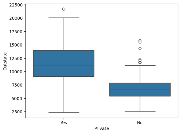
d. Now, produce a side-by-side boxplots of Outstate versus Private.
# Write your code below to answer the question
Compare your answer with the reference solution below
import seaborn as sns

sns.boxplot(x=college_df["Private"], y=college_df["Outstate"])

# From the box plot, we can state that for an outstate range of 9000 to 13500, we can get Private = Yes, and for the range from 5500 to 7500, we get Private = No.
<Axes: xlabel='Private', ylabel='Outstate'>
e. How many quantitative and qualitative features are there in this dataset?
# Write your code below to answer the question
Compare your answer with the reference solution below
import numpy as np

print(
    "The number of quantitative features in this dataset is %d and the number of qualitative features in this dataset is %d."
    % (
        college_df.select_dtypes(include=np.number).shape[1],
        college_df.select_dtypes(include=object).shape[1],
    )
)
The number of quantitative features in this dataset is 17 and the number of qualitative features in this dataset is 1.
f. Create a new qualitative variable, called Elite, by binning the Top10perc variable. We are going to divide universities into two groups based on whether or not the proportion of students coming from the top \(10\)% of their high school classes exceeds \(50\)%. Now see how many elite universities there are.
# Write your code below to answer the question
Compare your answer with the reference solution below
college_df["Elite"] = college_df["Top10perc"] > 50
college_df["Elite"].sum()
78
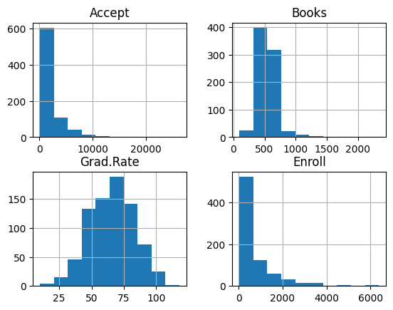
e. Use the hist() function to produce histogram of any \(4\) variables/features from the dataset chosen by you.
# Write your code below to answer the question
Compare your answer with the reference solution below
from matplotlib import pyplot as plt

college_df.hist(column=["Accept", "Books", "Grad.Rate", "Enroll"])
plt.show()

# We chose Accept, Books, Grad.Rate and Enroll features where the count for every features value is shown with a histogram which indicates the most frequent values for every feature.
f. Continue exploring the data, and provide a brief summary of what you discover.
# Write your code below to continue exploring the data