8.1. Generalised linear models¶

This section will focus on poisson regression, which is a generalised linear model (GLM) for count data.

8.1.1. Count data¶

In previous chapters, we learnt about linear regression for predicting quantitative (continuous) variables and logistic regression for predicting qualitative (categorical) variables. In this section, we will learn about regression for predicting count data. Count data is a special type of discrete data, where the values are non-negative integers. Examples of count data include the number of cars passing a toll booth, the number of people in a room, the number of times a word appears in a document, the number of times a user clicks on a link, and the number of times a user purchases a product.

To study the problem of predicting count data, we will use the Bikeshare dataset. The response is bikers, the number of hourly users of a bike sharing program in Washington, DC. Thus, this response variable is neither qualitative nor quantitative. Instead, it takes on non-negative integer values, or counts. We will consider predicting bikers using the features mnth (month of the year), hr (hour of the day, from 0 to 23), workingday (an indicator variable that equals 1 if it is neither a weekend nor a holiday), temp (the normalised temperature, in Celsius), and weathersit (a qualitative variable that takes on one of four possible values: clear; misty or cloudy; light rain or light snow; or heavy rain or heavy snow).

Get ready by importing the APIs needed from respective libraries.

import pandas as pd
import numpy as np
import matplotlib.pyplot as plt
import seaborn as sns

from statsmodels.formula.api import ols, poisson

%matplotlib inline

Load the data, indicate the type of the mnth and hr features, and display the first few rows.

data_url = "https://github.com/pykale/transparentML/raw/main/data/Bikeshare.csv"

data_df = pd.read_csv(data_url, header=0, index_col=0)
data_df["mnth"] = data_df["mnth"].astype("category")
data_df["hr"] = data_df["hr"].astype("category")
data_df.head(3)

	mnth	day	hr	holiday	weekday	workingday	weathersit	temp	atemp	hum	windspeed	casual	registered	bikers
season
1	Jan	1	0	0	6	0	clear	0.24	0.2879	0.81	0.0	3	13	16
1	Jan	1	1	0	6	0	clear	0.22	0.2727	0.80	0.0	8	32	40
1	Jan	1	2	0	6	0	clear	0.22	0.2727	0.80	0.0	5	27	32

8.1.2. Linear regression for predicting the number of bikers¶

As in the case of motivating logistic regression, let us predict bikers using linear regression first using the ols function from the statsmodels library. We will use the mnth, hr, workingday, temp, and weathersit features as predictors.

est = ols("bikers ~ mnth + hr + temp + workingday + weathersit", data_df).fit()
est.summary()

OLS Regression Results
Dep. Variable:	bikers	R-squared:	0.675
Model:	OLS	Adj. R-squared:	0.673
Method:	Least Squares	F-statistic:	457.3
Date:	Tue, 06 Feb 2024	Prob (F-statistic):	0.00
Time:	20:21:56	Log-Likelihood:	-49743.
No. Observations:	8645	AIC:	9.957e+04
Df Residuals:	8605	BIC:	9.985e+04
Df Model:	39
Covariance Type:	nonrobust

	coef	std err	t	P>\|t\|	[0.025	0.975]
Intercept	-27.2068	6.715	-4.052	0.000	-40.370	-14.044
mnth[T.Aug]	11.8181	4.698	2.515	0.012	2.609	21.028
mnth[T.Dec]	5.0328	4.280	1.176	0.240	-3.357	13.423
mnth[T.Feb]	-34.5797	4.575	-7.558	0.000	-43.548	-25.611
mnth[T.Jan]	-41.4249	4.972	-8.331	0.000	-51.172	-31.678
mnth[T.July]	3.8996	5.003	0.779	0.436	-5.907	13.706
mnth[T.June]	26.3938	4.642	5.686	0.000	17.294	35.493
mnth[T.March]	-24.8735	4.277	-5.815	0.000	-33.258	-16.489
mnth[T.May]	31.1322	4.150	7.501	0.000	22.997	39.268
mnth[T.Nov]	18.8851	4.099	4.607	0.000	10.850	26.920
mnth[T.Oct]	34.4093	4.006	8.589	0.000	26.556	42.262
mnth[T.Sept]	25.2534	4.293	5.883	0.000	16.839	33.668
hr[T.1]	-14.5793	5.699	-2.558	0.011	-25.750	-3.408
hr[T.2]	-21.5791	5.733	-3.764	0.000	-32.817	-10.341
hr[T.3]	-31.1408	5.778	-5.389	0.000	-42.468	-19.814
hr[T.4]	-36.9075	5.802	-6.361	0.000	-48.281	-25.534
hr[T.5]	-24.1355	5.737	-4.207	0.000	-35.381	-12.890
hr[T.6]	20.5997	5.704	3.612	0.000	9.419	31.781
hr[T.7]	120.0931	5.693	21.095	0.000	108.934	131.253
hr[T.8]	223.6619	5.690	39.310	0.000	212.509	234.815
hr[T.9]	120.5819	5.693	21.182	0.000	109.423	131.741
hr[T.10]	83.8013	5.705	14.689	0.000	72.618	94.985
hr[T.11]	105.4234	5.722	18.424	0.000	94.207	116.640
hr[T.12]	137.2837	5.740	23.916	0.000	126.032	148.536
hr[T.13]	136.0359	5.760	23.617	0.000	124.745	147.327
hr[T.14]	126.6361	5.776	21.923	0.000	115.313	137.959
hr[T.15]	132.0865	5.780	22.852	0.000	120.756	143.417
hr[T.16]	178.5206	5.772	30.927	0.000	167.206	189.836
hr[T.17]	296.2670	5.749	51.537	0.000	284.998	307.536
hr[T.18]	269.4409	5.736	46.976	0.000	258.198	280.684
hr[T.19]	186.2558	5.714	32.596	0.000	175.055	197.457
hr[T.20]	125.5492	5.704	22.012	0.000	114.369	136.730
hr[T.21]	87.5537	5.693	15.378	0.000	76.393	98.714
hr[T.22]	59.1226	5.689	10.392	0.000	47.970	70.275
hr[T.23]	26.8376	5.688	4.719	0.000	15.688	37.987
weathersit[T.cloudy/misty]	-12.8903	1.964	-6.562	0.000	-16.741	-9.040
weathersit[T.heavy rain/snow]	-109.7446	76.667	-1.431	0.152	-260.031	40.542
weathersit[T.light rain/snow]	-66.4944	2.965	-22.425	0.000	-72.307	-60.682
temp	157.2094	10.261	15.321	0.000	137.095	177.324
workingday	1.2696	1.784	0.711	0.477	-2.228	4.768

Omnibus:	288.526	Durbin-Watson:	0.519
Prob(Omnibus):	0.000	Jarque-Bera (JB):	518.512
Skew:	0.273	Prob(JB):	2.55e-113
Kurtosis:	4.068	Cond. No.	131.

Notes:
[1] Standard Errors assume that the covariance matrix of the errors is correctly specified.

From the above, we can see that a progression of weather from clear to cloudy results in 12.89 fewer bikers per hour on average. If the weather progresses further (from cloudy) to light rain or snow, then this further results in \(-12.89 - (-66.49) = 53.60\) fewer bikers per hour.

Let us study the coefficients of the mnth and hr features to understand the effect of these features on the response.

# months = ["Jan", "Feb", "March", "April", "May", "June", "July", "Aug", "Sept", "Oct", "Nov", "Dec"]
months = [
    "Jan",
    "Feb",
    "March",
    "May",
    "June",
    "July",
    "Aug",
    "Sept",
    "Oct",
    "Nov",
    "Dec",
]
coef_mnth = [est.params["mnth[T.%s]" % _m] for _m in months]
coef_hr = [est.params["hr[T.%d]" % _h] for _h in range(1, 24)]

Visualise the coefficients of the mnth and hr features using plots.

fig, (ax1, ax2) = plt.subplots(1, 2, figsize=(12, 5))
ax1.plot(months, coef_mnth, "bo-")
ax1.grid()
ax1.set_xlabel("Month")
ax2.plot(np.arange(1, 24), coef_hr, "bo-")
ax2.grid()
ax2.set_xlabel("Hour")

for ax in fig.axes:
    ax.set_ylabel("Coefficient")

plt.show()

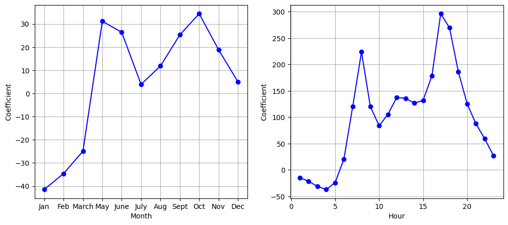
From the above figures, we can see that bike usage is highest in the spring and fall, and lowest during the winter months. Furthermore, bike usage is greatest around rush hour (9 AM and 6 PM), and lowest overnight. Thus, at first glance, fitting a linear regression model to the Bikeshare dataset seems to provide reasonable and intuitive results.

Let us examine the distribution of the estimated response values. We will use the predict function from the statsmodels library to obtain the predicted values.

fig = plt.figure(figsize=(12, 7))
y_pred = est.predict(data_df.loc[:, ["mnth", "hr", "temp", "workingday", "weathersit"]])
sns.histplot(y_pred, kde=True)
plt.show()

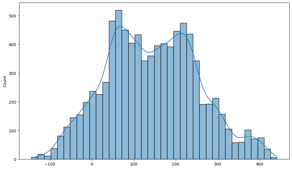
By careful inspection, we can identify several issues from the figure above, e.g. 9.6% of the fitted values are negative! Thus, the linear regression model predicts a negative number of users during 9.6% of the hours in the dataset, which does not make sense. Furthermore, the fitted values are not integers, which is also not desirable.

This casts doubt on the suitability of linear regression for performing meaningful predictions on the Bikeshare data. It also raises concerns about the accuracy of the coefficient estimates, confidence intervals, and other outputs of the regression model.

Let us further examine the distribution of the response variable bikers against the hr feature using the original scale and the log scale.

fig, (ax1, ax2) = plt.subplots(1, 2, figsize=(25, 7))

sns.stripplot(data=data_df, x="hr", y="bikers", ax=ax1, alpha=0.1, color=".2")
sns.boxplot(
    data=data_df,
    x="hr",
    y="bikers",
    ax=ax1,
    width=0.9,
    palette="vlag",
    meanline=True,
    showmeans=True,
)
ax1.set_ylabel("Number of Bikers")

sns.stripplot(data=data_df, x="hr", y="bikers", ax=ax2, alpha=0.1, color=".2")
sns.boxplot(
    data=data_df,
    x="hr",
    y="bikers",
    ax=ax2,
    width=0.9,
    palette="vlag",
    meanline=True,
    showmeans=True,
)
ax2.set_yscale("log")
ax2.set_ylabel("log(Number of Bikers)")
for ax in fig.axes:
    ax.set_xlabel("Hour")
plt.show()

/tmp/ipykernel_2418/623161877.py:4: FutureWarning: 

Passing `palette` without assigning `hue` is deprecated and will be removed in v0.14.0. Assign the `x` variable to `hue` and set `legend=False` for the same effect.

  sns.boxplot(

/tmp/ipykernel_2418/623161877.py:17: FutureWarning: 

Passing `palette` without assigning `hue` is deprecated and will be removed in v0.14.0. Assign the `x` variable to `hue` and set `legend=False` for the same effect.

  sns.boxplot(

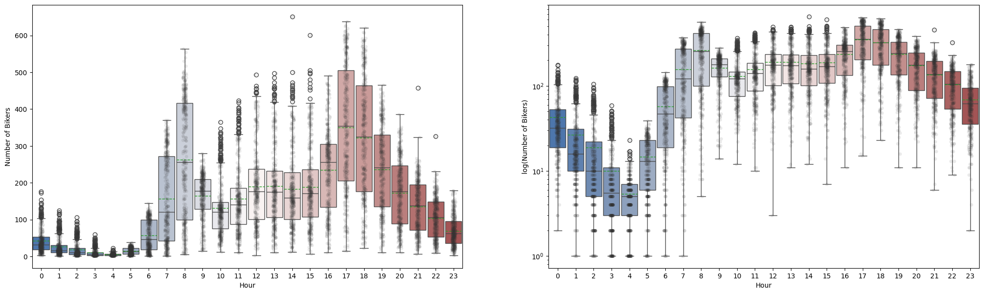
This figure corresponds to Figure 4.14 in the textbook. Intuitively, when the expected number of bikers is small, its variance should be small as well. For example, at 2 AM during a heavy December snow storm, we expect that extremely few people will use a bike, and moreover that there should be little variance associated with the number of users during those conditions. This is borne out in the data: between 1 AM and 4 AM, in December, January, and February, when it is raining, there are 5.05 users, on average, with a standard deviation of 3.73. By contrast, between 7 AM and 10 AM, in April, May, and June, when skies are clear, there are 243.59 users, on average, with a standard deviation of 131.7. The mean-variance relationship is displayed in the left-hand panel of the figure above. This is a major violation of the assumptions of a linear model, which state that \(y = \sum_{d=1}^{D}x_d\beta_d + \epsilon\), where \(\epsilon\) is a mean-zero error term with variance \(\sigma^2\) that is constant, and not a function of the features (covariates). Therefore, the heteroscedasticity of the data calls into question the suitability of a linear regression model.

Finally, the response bikers is integer-valued. But under a linear model, \(y = \beta_0 + \sum_{d=1}^{D}x_d\beta_d + \epsilon\), where \(\epsilon\) is a continuous-valued error term. This means that in a linear model, the response \(y\) is necessarily continuous-valued (quantitative). Thus, the integer nature of the response bikers suggests that a linear regression model is not entirely satisfactory for this dataset.

Some of the problems that arise when fitting a linear regression model to the Bikeshare data can be overcome by transforming the response; for instance, we can fit the model

\[ \log(y) = \beta_0 + \sum_{d=1}^{D}x_d\beta_d + \epsilon. \]

Transforming the response avoids the possibility of negative predictions, and it overcomes much of the heteroscedasticity in the untransformed data, as is shown in the right-hand panel of the figure above.

However, it is not quite a satisfactory solution, since predictions and inference are made in terms of the log of the response, rather than the response. This leads to challenges in interpretation, e.g. a one-unit increase in \(x_d\) is associated with an increase in the mean of the log of \(y\) by an amount \(\beta_d\). Furthermore, a log transformation of the response cannot be applied in settings where the response can take on a value of 0. Thus, while fitting a linear model to a transformation of the response may be an adequate approach for some count-valued datasets, it often leaves something to be desired. This motivates the development of a Poisson regression model that provides a much more natural and elegant approach for this task.

8.1.3. Poisson regression for predicting the number of bikers¶

To overcome the inadequacies of linear regression for analysing the Bikeshare dataset, we will study a GLM approach called Poisson regression.

8.1.3.1. The Poisson distribution¶

Let us first introduce the Poisson distribution. Suppose that a random variable \(y\) takes on nonnegative integer values, i.e. \(y \in \{0, 1, 2, \dots\}\). If \(y\) follows the Poisson distribution, then

(8.1)¶\[\mathbb{P}(y=t) = \frac{\lambda^t e^{-\lambda}}{t!}, \quad t = 0, 1, 2, \dots .\]

Here, \(\lambda>0\) is a positive real number, called the rate parameter, which is the expected value of \(y\), i.e. \(\mathbb{E}(y)\). It turns out that \(\lambda\) also equals the variance of \(y\), i.e. \(λ = \mathbb{E}(y) = \text{Var}(y)\). This means that if \(y\) follows the Poisson distribution, then the larger the mean of \(y\) , the larger its variance. The notation \( t! \) in Equation (8.1) denotes the factorial of \(t\), i.e. \( t! = t \times (t − 1) \times (t − 2) \times \cdots \times 3 \times 2 \times 1\). The Poisson distribution is typically used to model counts, a natural choice since counts, like the Poisson distribution, take on non-negative integer values.

How to interpret the Poisson distribution?

To see how we might use the Poisson distribution in practice, let \(y\) denote the number of users of the bike sharing programme during a particular hour of the day, under a particular set of weather conditions, and during a particular month of the year. We can model \(y\) as a Poisson distribution with mean \(\mathbb{E}(y) = \lambda = 5\). This means that the probability of no users during this particular hour is \(\mathbb{P}(y = 0) = \frac{e^{-5}5^0}{0!} = e^{-5} = 0.0067 \), where 0! = 1 by convention. The probability that there is exactly one user is \( \mathbb{P}(y = 1) = \frac{e^{-5}5^1}{1!} = 0.034 \), the probability of two users is \( \mathbb{P}(y = 2) = \frac{e^{-5}5^2}{2!} = 0.084 \) and so on.

8.1.3.2. The Poisson regression model¶

In reality, we expect the mean number of users of the bike sharing program, \( \lambda = \mathbb{E}(y) \), to vary as a function of the hour of the day, the month of the year, the weather conditions, and so forth. So rather than modelling the number of bikers, \(y\) , as a Poisson distribution with a fixed mean value like \(\lambda = 5 \), we would like to allow the mean to vary as a function of the features (covariates). In particular, we consider the following model for the mean \( \lambda = \mathbb{E}(y) \), which we now write as \( \lambda(x_1, \cdots, x_D) \) to emphasise that it is a function of the features \( x_1, \cdots, x_D \):

\[ \log(\lambda(x_1, \cdots, x_D)) = \beta_0 + \sum_{d=1}^{D}x_d\beta_d. \]

or equivalently,

(8.2)¶\[\lambda(x_1, \cdots, x_D) = e^{\beta_0 + \sum_{d=1}^{D}x_d\beta_d}.\]

Here, \( \beta_0, \beta_1, \cdots, \beta_D \) are parameters to be estimated. Together, the above equations define the Poisson regression model.

To estimate the coefficients (parameters) \( \beta_0, \beta_1, \cdots, \beta_D \), we use the same maximum likelihood approach that we adopted for logistic regression. The likelihood function for the Poisson regression model is

\[ \ell(\beta_0, \beta_1, \cdots, \beta_D) = \prod_{n=1}^{N} \frac{\lambda(\mathbf{x}_n)^{y_n} e^{-\lambda(\mathbf{x}_n)}}{y_n!}, \]

where \(\lambda(\mathbf{x}_n) = e^{\beta_0 + \sum_{d=1}^{D}x_{nd}\beta_d}\), and \(y_n\) is the response for the \(n\text{th}\) sample (observation). We obtain the coefficient estimates as those maximise the likelihood \(\ell(\beta_0, \beta_1, \cdots, \beta_D)\), i.e. those make the observed data as likely as possible.

We now fit a Poisson regression model to the Bikeshare dataset using the statsmodels package.

est = poisson("bikers ~ mnth + hr + temp + workingday + weathersit", data_df).fit()
est.summary()

Optimization terminated successfully.
         Current function value: 16.256725
         Iterations 9

Poisson Regression Results
Dep. Variable:	bikers	No. Observations:	8645
Model:	Poisson	Df Residuals:	8605
Method:	MLE	Df Model:	39
Date:	Tue, 06 Feb 2024	Pseudo R-squ.:	0.7459
Time:	20:21:58	Log-Likelihood:	-1.4054e+05
converged:	True	LL-Null:	-5.5298e+05
Covariance Type:	nonrobust	LLR p-value:	0.000

	coef	std err	z	P>\|z\|	[0.025	0.975]
Intercept	3.3854	0.010	333.686	0.000	3.365	3.405
mnth[T.Aug]	0.1296	0.005	26.303	0.000	0.120	0.139
mnth[T.Dec]	-0.0048	0.005	-0.951	0.342	-0.015	0.005
mnth[T.Feb]	-0.4656	0.006	-76.909	0.000	-0.478	-0.454
mnth[T.Jan]	-0.6917	0.007	-98.996	0.000	-0.705	-0.678
mnth[T.July]	0.0821	0.005	15.545	0.000	0.072	0.092
mnth[T.June]	0.2017	0.005	41.673	0.000	0.192	0.211
mnth[T.March]	-0.3153	0.005	-58.225	0.000	-0.326	-0.305
mnth[T.May]	0.2189	0.004	49.792	0.000	0.210	0.228
mnth[T.Nov]	0.1287	0.005	27.880	0.000	0.120	0.138
mnth[T.Oct]	0.2460	0.004	56.949	0.000	0.238	0.255
mnth[T.Sept]	0.2120	0.005	46.873	0.000	0.203	0.221
hr[T.1]	-0.4716	0.013	-36.278	0.000	-0.497	-0.446
hr[T.2]	-0.8088	0.015	-55.220	0.000	-0.837	-0.780
hr[T.3]	-1.4439	0.019	-76.631	0.000	-1.481	-1.407
hr[T.4]	-2.0761	0.025	-83.728	0.000	-2.125	-2.027
hr[T.5]	-1.0603	0.016	-65.957	0.000	-1.092	-1.029
hr[T.6]	0.3245	0.011	30.585	0.000	0.304	0.345
hr[T.7]	1.3296	0.009	146.822	0.000	1.312	1.347
hr[T.8]	1.8313	0.009	211.630	0.000	1.814	1.848
hr[T.9]	1.3362	0.009	148.191	0.000	1.318	1.354
hr[T.10]	1.0912	0.009	117.831	0.000	1.073	1.109
hr[T.11]	1.2485	0.009	137.304	0.000	1.231	1.266
hr[T.12]	1.4340	0.009	160.486	0.000	1.417	1.452
hr[T.13]	1.4280	0.009	159.529	0.000	1.410	1.445
hr[T.14]	1.3793	0.009	153.266	0.000	1.362	1.397
hr[T.15]	1.4081	0.009	156.862	0.000	1.391	1.426
hr[T.16]	1.6287	0.009	184.979	0.000	1.611	1.646
hr[T.17]	2.0490	0.009	239.221	0.000	2.032	2.066
hr[T.18]	1.9667	0.009	229.065	0.000	1.950	1.983
hr[T.19]	1.6684	0.009	190.830	0.000	1.651	1.686
hr[T.20]	1.3706	0.009	152.737	0.000	1.353	1.388
hr[T.21]	1.1186	0.009	121.383	0.000	1.101	1.137
hr[T.22]	0.8719	0.010	91.429	0.000	0.853	0.891
hr[T.23]	0.4814	0.010	47.164	0.000	0.461	0.501
weathersit[T.cloudy/misty]	-0.0752	0.002	-34.528	0.000	-0.080	-0.071
weathersit[T.heavy rain/snow]	-0.9263	0.167	-5.554	0.000	-1.253	-0.599
weathersit[T.light rain/snow]	-0.5758	0.004	-141.905	0.000	-0.584	-0.568
temp	0.7853	0.011	68.434	0.000	0.763	0.808
workingday	0.0147	0.002	7.502	0.000	0.011	0.018

Let us do the same plots as before to visualise the relationship between the number of bikers and the features mnth and hr.

fig, (ax1, ax2) = plt.subplots(1, 2, figsize=(12, 5))
ax1.plot(months, coef_mnth, "bo-")
ax1.grid()
ax1.set_xlabel("Month")
ax2.plot(np.arange(1, 24), coef_hr, "bo-")
ax2.grid()
ax2.set_xlabel("Hour")

for ax in fig.axes:
    ax.set_ylabel("Coefficient")

plt.show()

We again see that bike usage is highest in the spring and fall and during rush hour, and lowest during the winter and in the early morning hours. In general, bike usage increases as the temperature increases, and decreases as the weather worsens. Interestingly, the coefficient associated with workingday is statistically significant under the Poisson regression model, but not under the linear regression model.

8.1.3.3. Key distinctions between Poisson and linear regression¶

Some important distinctions between the Poisson regression model and the linear regression model are as follows:

Interpretation: To interpret the coefficients in the Poisson regression model, we must pay close attention to Equation (8.2), which states that an increase in \(x_d\) by one unit is associated with a change in \(\mathbb{E}(y) = \lambda\) by a factor of \(\textrm{exp}(\beta_d)\). For example, a change in weather from clear to cloudy skies is associated with a change in mean bike usage by a factor of \(\textrm{exp}(−0.08) = 0.923\), i.e. on average, only 92.3% as many people will use bikes when it is cloudy relative to when it is clear. If the weather worsens further and it begins to rain, then the mean bike usage will further change by a factor of \( \textrm{exp} (−0.5) = 0.607\), i.e. on average only 60.7% as many people will use bikes when it is rainy relative to when it is cloudy.
Mean-variance relationship: As mentioned earlier, under the Poisson model, \( \lambda = \mathbb{E}(y) = \text{Var}(y) \). Thus, by modelling bike usage with a Poisson regression, we implicitly assume that mean bike usage in a given hour equals the variance of bike usage during that hour. By contrast, under a linear regression model, the variance of bike usage always takes on a constant value. From the above figure (the one corresponding to Figure 4.14 in the textbook), in the Bikeshare data, when biking conditions are favourable, both the mean and the variance in bike usage are much higher than when conditions are unfavourable. Thus, the Poisson regression model is able to handle the mean-variance relationship seen in the Bikeshare data in a way that the linear regression model is not.
Nonnegative fitted values: There are no negative predictions using the Poisson regression model. This is because the Poisson model itself only allows for nonnegative values, as shown in Equation (8.1). By contrast, when we fit a linear regression model to the Bikeshare dataset, almost 10% of the predictions were negative.

8.1.4. GLM characteristics¶

Based on the two GLM models we have seen so far, the logistic regression model and the Poisson regression model, we can summarise the common characteristics of GLMs as follows:

Each approach uses features (predictors) \( x_1, x_2, \dots, x_D \) to predict a response (output) \( y \). We assume that, conditional on \( x_1, x_2,\dots, x_D \), \( y \) belongs to a certain family of distributions. For linear regression, we typically assume that \(y\) follows a Gaussian (normal) distribution. For logistic regression, we assume that \(y\) follows a Bernoulli distribution. Finally, for Poisson regression, we assume that \(y\) follows a Poisson distribution.
Each approach models the mean (expectation) of \(y\) as a function of the features (predictors). In linear regression, the mean of \(y\) takes the form

\[ \mathbb{E}(y|x_1, x_2, \dots, x_D) = \beta_0 + \beta_1 x_1 + \cdots + \beta_p x_D. \]

In logistic regression, the mean of \(y\) takes the form

\[ \mathbb{E}(y|x_1, x_2, \dots, x_D) = \mathbb{P}(y=1|x_1, x_2, \dots, x_D) = \frac{e^{\beta_0 + \beta_1 x_1 + \cdots + \beta_p x_D}}{1 + e^{\beta_0 + \beta_1 x_1 + \cdots + \beta_p x_D}}. \]

In Poisson regression, it takes the form

\[ \mathbb{E}(y|x_1, x_2, \dots, x_D) = \lambda(x_1, x_2, \dots, x_D) = e^{\beta_0 + \beta_1 x_1 + \cdots + \beta_p x_D}. \]

The above three equations can be expressed using a link function, \( \eta \), which applies a transformation to \( \mathbb{E}(y|x_1, x_2, \dots, x_D) \) so that the transformed mean is a linear function of the features (predictors). That is

(8.3)¶\[\eta(\mathbb{E}(y|x_1, x_2, \dots, x_D)) = \beta_0 + \beta_1 x_1 + \cdots + \beta_p x_D.\]

The link functions for linear, logistic and Poisson regression are \(\eta(\mu) = \mu \), \( \eta(\mu) = \log(\mu/(1 − \mu)) \), and \(\eta(\mu) = \log(\mu)\), respectively.

The Gaussian, Bernoulli and Poisson distributions are all members of a wider class of distributions, known as the exponential family. Other well known members of this family are the exponential distribution, the Gamma distribution, and the negative binomial distribution. In general, we can perform a regression by modelling the response \(y\) as coming from a particular member of the exponential family, and then transforming the mean of the response so that the transformed mean is a linear function of the features (predictors) via the link function above in Equation (8.3). Any regression approach that follows this very general recipe is known as a generalized linear model (GLM). Thus, linear regression, logistic regression, and Poisson regression are three examples of GLMs. Other examples not covered here include Gamma regression and negative binomial regression.

8.1.5. Exercises¶

1. Logistic regression is a generalised linear model (GLM).

   a. True

   b. False

Compare your answer with the solution below

b. True.

2. There are no negative predictions using the Poisson regression model.

   a. True

   b. False

Compare your answer with the solution below

b. True.

3. For linear regression, we typically assume that \(y\) (output) follows a Bernoulli distribution.

   a. True

   b. False

Compare your answer with the solution below

b. False. Linear regression assumes that the output (\(y\)) follows a Gaussian(normal) distribution

Transparent ML Intro

Generalised linear models

Contents

8.1. Generalised linear models¶

8.1.1. Count data¶

8.1.2. Linear regression for predicting the number of bikers¶

8.1.3. Poisson regression for predicting the number of bikers¶

8.1.3.1. The Poisson distribution¶

8.1.3.2. The Poisson regression model¶

8.1.3.3. Key distinctions between Poisson and linear regression¶

8.1.4. GLM characteristics¶

8.1.5. Exercises¶