7.2. Classification trees¶

Classification trees are very similar to regression trees, except that the target variable is categorical. In regression trees, we used the mean of the target variable in each region as the prediction. In classification trees, we use the most common class in each region as the prediction. Besides the most common class, we are also interested in the proportion of each class in each region. This is because the proportion of each class in each region is a measure of the purity of the region. A region is pure if it contains only one class. A region is impure if it contains multiple classes.

7.2.1. Gini index¶

Although classification accuracy is a good measure for classification performance, a popular cost function (splitting criterion) for classification trees is the Gini index, a measure of the impurity of a region (not just feature regions in machine learning, but also regions in society in economics, e.g. to measure income/wealth inequality). This is because classification accuracy is not sufficiently sensitive for building classification trees.

The Gini index is defined as:

\[ G = 1 - \sum_{c=1}^C p_c^2 = \sum_{c=1}^C p_c (1 - p_c), \]

where \(p_c\) is the proportion of class \(c\) in the region. The Gini index is zero if the region is pure, and is one if the region is impure. The Gini index is a measure of the probability of misclassification. The Gini index is also known as the Gini impurity.

7.2.2. Entropy¶

Another popular cost function (splitting criterion) for classification trees is the entropy, which is defined as:

\[ H = - \sum_{c=1}^C p_c \log_2 p_c, \]

where \(p_c\) is the proportion of class \(c\) in the region. The entropy is zero if the region is pure, and is one if the region is impure.

When building classification trees, either the Gini index or the entropy are typically used to evaluate the quality of a particular split, and the split that produces the lowest cost is chosen. The Gini index and the entropy are very similar, and the Gini index is slightly faster to compute.

7.2.3. Classification trees for heart disease diagnosis¶

Get ready by importing the APIs needed from respective libraries.

import numpy as np
import pandas as pd
from sklearn.model_selection import train_test_split
from sklearn.tree import DecisionTreeClassifier, plot_tree
from sklearn.metrics import confusion_matrix, accuracy_score, classification_report
import matplotlib.pyplot as plt

%matplotlib inline

Set a random seed for reproducibility.

np.random.seed(2022)

We use the Heart dataset (click to explore) to predict whether a patient has heart disease or not. The target variable is AHD, which is a binary variable that indicates whether a patient has heart disease or not.

Load the dataset and remove the rows with missing values. Inspect the first few rows of the dataset.

heart_url = "https://github.com/pykale/transparentML/raw/main/data/Heart.csv"

heart_df = pd.read_csv(heart_url).dropna()
heart_df.head()

	Unnamed: 0	Age	Sex	ChestPain	RestBP	Chol	Fbs	RestECG	MaxHR	ExAng	Oldpeak	Slope	Ca	Thal	AHD
0	1	63	1	typical	145	233	1	2	150	0	2.3	3	0.0	fixed	No
1	2	67	1	asymptomatic	160	286	0	2	108	1	1.5	2	3.0	normal	Yes
2	3	67	1	asymptomatic	120	229	0	2	129	1	2.6	2	2.0	reversable	Yes
3	4	37	1	nonanginal	130	250	0	0	187	0	3.5	3	0.0	normal	No
4	5	41	0	nontypical	130	204	0	2	172	0	1.4	1	0.0	normal	No

Take a look at the structure of the dataset.

heart_df.info()

<class 'pandas.core.frame.DataFrame'>
Index: 297 entries, 0 to 301
Data columns (total 15 columns):
 #   Column      Non-Null Count  Dtype  
---  ------      --------------  -----  
 0   Unnamed: 0  297 non-null    int64  
 1   Age         297 non-null    int64  
 2   Sex         297 non-null    int64  
 3   ChestPain   297 non-null    object 
 4   RestBP      297 non-null    int64  
 5   Chol        297 non-null    int64  
 6   Fbs         297 non-null    int64  
 7   RestECG     297 non-null    int64  
 8   MaxHR       297 non-null    int64  
 9   ExAng       297 non-null    int64  
 10  Oldpeak     297 non-null    float64
 11  Slope       297 non-null    int64  
 12  Ca          297 non-null    float64
 13  Thal        297 non-null    object 
 14  AHD         297 non-null    object 
dtypes: float64(2), int64(10), object(3)
memory usage: 37.1+ KB

Use the factorize method from the pandas library to convert categorical variables to numerical variables. This is because the sklearn library only accepts numerical variables. ChestPain is a categorical variable that indicates the type of chest pain. Thal is a categorical variable that indicates the type of thalassemia.

heart_df.ChestPain = pd.factorize(heart_df.ChestPain)[0]
heart_df.Thal = pd.factorize(heart_df.Thal)[0]

Get the feature matrix X and the target vector y.

X = heart_df.drop("AHD", axis=1)
y = pd.factorize(heart_df.AHD)[0]

Fit a classification tree to the data using the DecisionTreeClassifier class from the sklearn.tree module. Set the max_leaf_nodes parameter to 6. This will limit the number of leaf nodes to 6. Set the max_features parameter to 3. This will limit the number of features to consider when looking for the best split to 3. It will randomly select these 3 features at each split.

clf = DecisionTreeClassifier(max_leaf_nodes=6, max_features=3)
clf.fit(X, y)

DecisionTreeClassifier(max_features=3, max_leaf_nodes=6)

In a Jupyter environment, please rerun this cell to show the HTML representation or trust the notebook.
On GitHub, the HTML representation is unable to render, please try loading this page with nbviewer.org.

Compute the accuracy of the classification tree on the training data.

clf.score(X, y)

0.8047138047138047

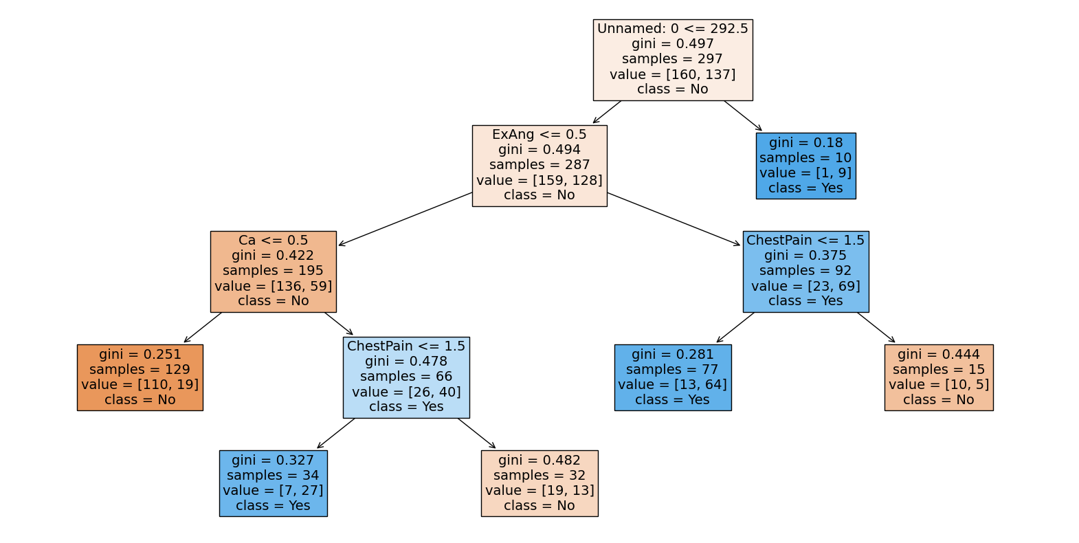
Visualise the classification tree using the plot_tree function from the sklearn.tree module. Set the filled parameter to True to colour the nodes in the tree according to the majority class in each region. Set the feature_names parameter to the list of feature names. Set the class_names parameter to the list of class names.

plt.figure(figsize=(20, 10))
plot_tree(
    clf, filled=True, feature_names=X.columns, class_names=["No", "Yes"], fontsize=14
)
plt.show()

../_images/classification-trees_17_0.png

7.2.4. Classification trees for car seat sales¶

Next, let us study the Carseats dataset (click to explore). In this dataset, we want to predict whether a car seat will be High or Low based on the Sales and Price of the car seat.

Load the dataset. Sales is a continuous variable so we recode it as a binary variable High by thresholding it at 8 using the map() function from the pandas library. High takes on a value of ‘Y’ if the Sales variable exceeds 8, ‘N’ otherwise. We also convert categorical variables to numerical variables using the factorize method from the pandas library as above.

Inspect the first few rows of the dataset.

carseats_url = "https://github.com/pykale/transparentML/raw/main/data/Carseats.csv"

carseats_df = pd.read_csv(carseats_url)
carseats_df["High"] = carseats_df.Sales.map(lambda x: "Y" if x > 8 else "N")
carseats_df.ShelveLoc = pd.factorize(carseats_df.ShelveLoc)[0]
carseats_df.Urban = carseats_df.Urban.map(lambda x: 1 if x == "Yes" else 0)
carseats_df.US = carseats_df.US.map(lambda x: 1 if x == "Yes" else 0)
carseats_df.head()

	Sales	CompPrice	Income	Advertising	Population	Price	ShelveLoc	Age	Education	Urban	US	High
0	9.50	138	73	11	276	120	0	42	17	1	1	Y
1	11.22	111	48	16	260	83	1	65	10	1	1	Y
2	10.06	113	35	10	269	80	2	59	12	1	1	Y
3	7.40	117	100	4	466	97	2	55	14	1	1	N
4	4.15	141	64	3	340	128	0	38	13	1	0	N

Take a look at the structure of the dataset.

carseats_df.info()

<class 'pandas.core.frame.DataFrame'>
RangeIndex: 400 entries, 0 to 399
Data columns (total 12 columns):
 #   Column       Non-Null Count  Dtype  
---  ------       --------------  -----  
 0   Sales        400 non-null    float64
 1   CompPrice    400 non-null    int64  
 2   Income       400 non-null    int64  
 3   Advertising  400 non-null    int64  
 4   Population   400 non-null    int64  
 5   Price        400 non-null    int64  
 6   ShelveLoc    400 non-null    int64  
 7   Age          400 non-null    int64  
 8   Education    400 non-null    int64  
 9   Urban        400 non-null    int64  
 10  US           400 non-null    int64  
 11  High         400 non-null    object 
dtypes: float64(1), int64(10), object(1)
memory usage: 37.6+ KB

Split the dataset into training (200 samples) and test sets.

X2 = carseats_df.drop(["Sales", "High"], axis=1)
y2 = carseats_df.High
train_size = 200
X_train, X_test, y_train, y_test = train_test_split(
    X2, y2, train_size=train_size, test_size=X.shape[0] - train_size
)

For this dataset, let us use ‘entropy’ as the split criterion at each node to fit a classification tree to the training data.

criteria = "entropy"
max_depth = 6
min_sample_leaf = 4
clf_gini = DecisionTreeClassifier(
    criterion=criteria, max_depth=max_depth, min_samples_leaf=min_sample_leaf
)
clf_gini.fit(X_train, y_train)
print(clf_gini.score(X_train, y_train))

0.895

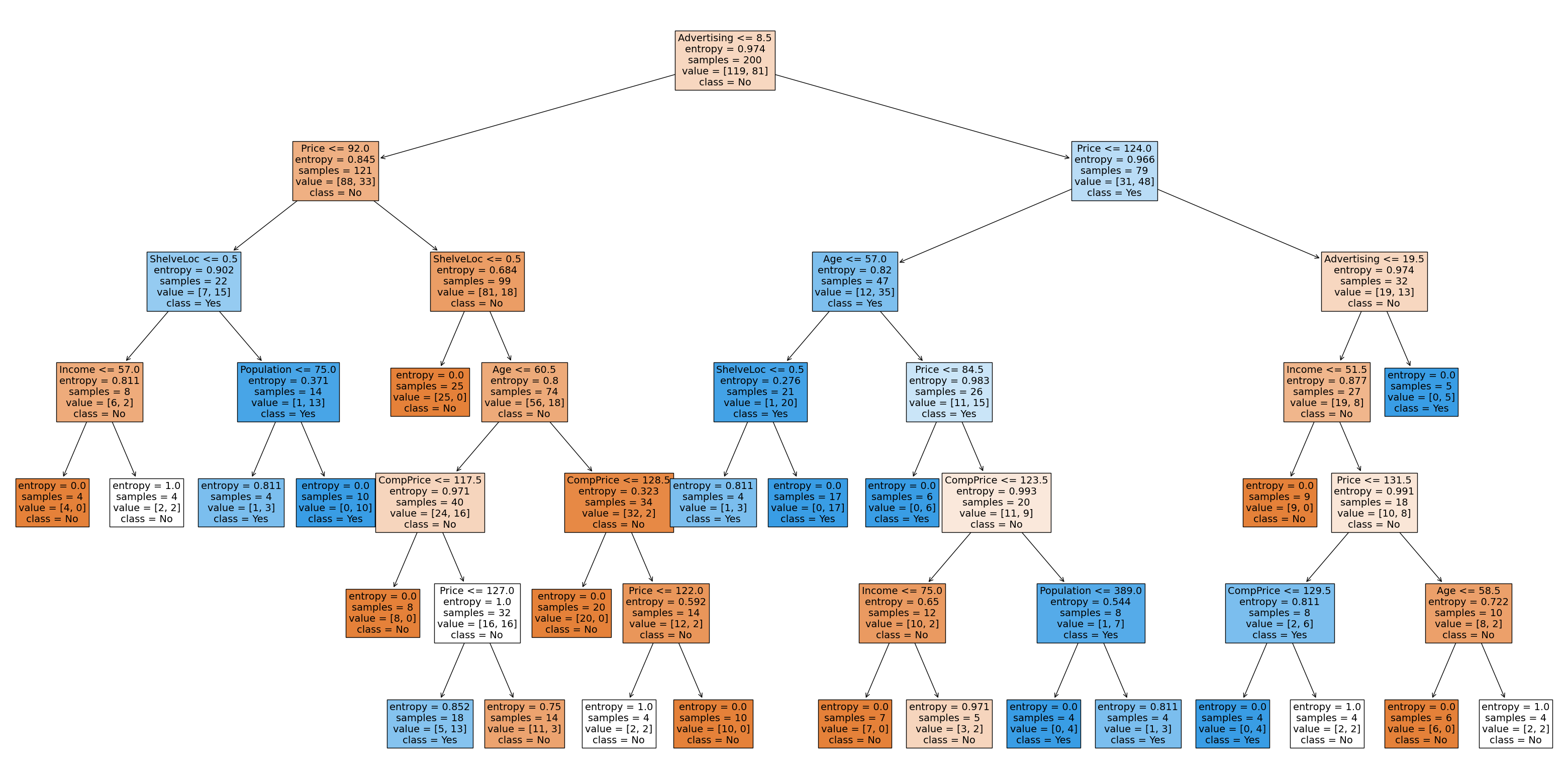
Visualise the classification tree.

# one attractive feature of a tree is visulization.
plt.figure(figsize=(40, 20))  # customize according to the size of your tree
plot_tree(
    clf_gini,
    filled=True,
    feature_names=X_train.columns,
    class_names=["No", "Yes"],
    fontsize=14,
)
plt.show()

../_images/classification-trees_27_0.png

Build the confusion matrix to evaluate the model in accuracy for both training and test datasets.

y_pred_train = clf_gini.predict(X_train)
cm = pd.DataFrame(
    confusion_matrix(y_train, y_pred_train).T,
    index=["No", "Yes"],
    columns=["No", "Yes"],
)
print(cm)
print("Train Accuracy is ", accuracy_score(y_train, y_pred_train) * 100)


y_pred = clf_gini.predict(X_test)
cm = pd.DataFrame(
    confusion_matrix(y_test, y_pred).T, index=["No", "Yes"], columns=["No", "Yes"]
)
print(cm)
print("Test Accuracy is ", accuracy_score(y_test, y_pred) * 100)

      No  Yes
No   111   13
Yes    8   68
Train Accuracy is  89.5
     No  Yes
No   46   15
Yes  13   23
Test Accuracy is  71.1340206185567

The test accuracy of the fitted model is significantly lower than the training accuracy, an indication of overfitting. You can go back and change the hyperparameters in the training process to reduce the dimension (flexibility) of the parameter space and reduce overfitting.

Compute more metrics such as precision, recall, f1-score, etc.

print(classification_report(y_test, y_pred))

              precision    recall  f1-score   support

           N       0.75      0.78      0.77        59
           Y       0.64      0.61      0.62        38

    accuracy                           0.71        97
   macro avg       0.70      0.69      0.69        97
weighted avg       0.71      0.71      0.71        97

7.2.5. Exercises¶

1. All the following exercises use the Caravan dataset.

Load the Caravan dataset and inspect the first five rows.

# Write your code below to answer the question

Compare your answer with the reference solution below

import pandas as pd

caravan_url = "https://github.com/pykale/transparentML/raw/main/data/Caravan.csv"
caravan_df = pd.read_csv(caravan_url)
caravan_df.head()

	MOSTYPE	MAANTHUI	MGEMOMV	MGEMLEEF	MOSHOOFD	MGODRK	MGODPR	MGODOV	MGODGE	MRELGE	...	ABRAND	Purchase
0	33	1	3	2	8	0	5	1	3	7	...	1	No
1	37	1	2	2	8	1	4	1	4	6	...	1	No
2	37	1	2	2	8	0	4	2	4	3	...	1	No
3	9	1	3	3	3	2	3	2	4	5	...	1	No
4	40	1	4	2	10	1	4	1	4	7	...	1	No

5 rows × 86 columns

2. Now, split the Caravan dataset into train and test sets using the proportion 80:20 and fit a DecisionTreeClassifier with \(8\) maximum leaf nodes and \(6\) maximum features. Calculate the testing accuracy and AUC of the fitted model. (Use \(2022\) as the random seed value)

# Write your code below to answer the question

Compare your answer with the reference solution below

import numpy as np
from sklearn.model_selection import train_test_split
from sklearn.tree import DecisionTreeClassifier, plot_tree
from sklearn.metrics import accuracy_score, roc_auc_score

np.random.seed(2022)

X2 = caravan_df.drop(["Purchase"], axis=1)
y2 = caravan_df.Purchase

X_train, X_test, y_train, y_test = train_test_split(X2, y2, test_size=0.20)

clf = DecisionTreeClassifier(max_leaf_nodes=8, max_features=6, random_state=2022)

clf.fit(X_train, y_train)


y_pred = clf.predict(X_test)
accuarcy = accuracy_score(y_test, y_pred)
print("Accuracy: ", accuarcy)


y_prob = clf.predict_proba(X_test)[:, 1]
roc_auc = roc_auc_score(y_test, y_prob)
print("AUC: ", roc_auc)

Accuracy:  0.9399141630901288
AUC:  0.5891454664057404

3. Now, train another DecisionTreeClassifier using entropy as the split criterion at each node to fit a classification tree with a maximum depth of \(4\) and a minimum sample leaf of \(3\) on the training data and find out the testing accuracy and AUC. (Use \(2022\) as the random seed value)

# Write your code below to answer the question

Compare your answer with the reference solution below

from sklearn.model_selection import train_test_split
from sklearn.tree import DecisionTreeClassifier, plot_tree

np.random.seed(2022)


criteria = "entropy"
max_depth = 4
min_sample_leaf = 3
clf_gini = DecisionTreeClassifier(
    criterion=criteria, max_depth=max_depth, min_samples_leaf=min_sample_leaf
)
clf_gini.fit(X_train, y_train)

y_pred = clf_gini.predict(X_test)
accuarcy = accuracy_score(y_test, y_pred)
print("Accuracy: ", accuarcy)


y_prob = clf_gini.predict_proba(X_test)[:, 1]
roc_auc = roc_auc_score(y_test, y_prob)
print("AUC: ", roc_auc)

Accuracy:  0.9399141630901288
AUC:  0.7402804957599478

4. Compare the performance of the trained models in Exercise 3 with Exercise 2.

Compare your answer with the solution below

In terms of testing accuracy, the Exercise 2 model outperformed the Exercise 3 model, but accuracy is not the only metric to evaluate the models. When we look at the AUC score, which more comprehensively evaluates a model in imbalanced tasks, the Exercise 3 model outperforms the Exercise 2 model. Therefore, in this case we can see the Exercise 3 model is better than the Exercise 2 model.

5. Create a confusion matrix and a classification report to help you evaluate the model you trained in Exercise 3.

# Write your code below to answer the question

Compare your answer with the reference solution below

from sklearn.metrics import confusion_matrix, classification_report

y_pred = clf_gini.predict(X_test)
cm = pd.DataFrame(
    confusion_matrix(y_test, y_pred).T, index=["No", "Yes"], columns=["No", "Yes"]
)
print("Confusion matrix\n", cm)

print(classification_report(y_test, y_pred))

Confusion matrix
        No  Yes
No   1093   68
Yes     2    2
              precision    recall  f1-score   support

          No       0.94      1.00      0.97      1095
         Yes       0.50      0.03      0.05        70

    accuracy                           0.94      1165
   macro avg       0.72      0.51      0.51      1165
weighted avg       0.91      0.94      0.91      1165

a. What is the testing accuracy of the model trained in Exercise 3?

Compare your answer with the solution below

The testing accuracy of the model trained in Exercise 3 is 0.94.

b. Does the model predicted well?

Compare your answer with the solution below

If we only consider the test accuracy, we may conclude that the model learned the task effectively, but this is not the whole story. In fact, due to the class imbalance in the training data, this model is biased towards the “NO” class. If we look at the confusion matrix, we see that it predicts “NO” for almost all samples, and has a poor recall and precision rate for the “YES” class. Again, this shows that accuracy alone is also not always a good metric for evaluating models. Considering AUC, recall, and precision as well as showing the confusion matrix, we can get a much better picture.

Transparent ML Intro

Classification trees

Contents

7.2. Classification trees¶

7.2.1. Gini index¶

7.2.2. Entropy¶

7.2.3. Classification trees for heart disease diagnosis¶

7.2.4. Classification trees for car seat sales¶

7.2.5. Exercises¶

	MOSTYPE	MAANTHUI	MGEMOMV	MGEMLEEF	MOSHOOFD	MGODRK	MGODPR	MGODOV	MGODGE	MRELGE	...	ABRAND	Purchase
0	33	1	3	2	8	0	5	1	3	7	...	1	No
1	37	1	2	2	8	1	4	1	4	6	...	1	No
2	37	1	2	2	8	0	4	2	4	3	...	1	No
3	9	1	3	3	3	2	3	2	4	5	...	1	No
4	40	1	4	2	10	1	4	1	4	7	...	1	No

	MOSTYPE	MAANTHUI	MGEMOMV	MGEMLEEF	MOSHOOFD	MGODRK	MGODPR	MGODOV	MGODGE	MRELGE	...	ABRAND	Purchase
0	33	1	3	2	8	0	5	1	3	7	...	1	No
1	37	1	2	2	8	1	4	1	4	6	...	1	No
2	37	1	2	2	8	0	4	2	4	3	...	1	No
3	9	1	3	3	3	2	3	2	4	5	...	1	No
4	40	1	4	2	10	1	4	1	4	7	...	1	No

	MOSTYPE	MAANTHUI	MGEMOMV	MGEMLEEF	MOSHOOFD	MGODRK	MGODPR	MGODOV	MGODGE	MRELGE	...	ABRAND	Purchase
0	33	1	3	2	8	0	5	1	3	7	...	1	No
1	37	1	2	2	8	1	4	1	4	6	...	1	No
2	37	1	2	2	8	0	4	2	4	3	...	1	No
3	9	1	3	3	3	2	3	2	4	5	...	1	No
4	40	1	4	2	10	1	4	1	4	7	...	1	No