Machine learning systems
Contents
1.2. Machine learning systems
Firstly, let us learn about the machine learning problems in their typical definitions.
1.2.1. Machine learning problems
Machine learning problems can be broadly classified into two categories: supervised learning and unsupervised learning. In supervised learning, the data is labelled, and the goal is to predict or estimate the label for new data. In unsupervised learning, the data is not labelled, and the goal is to find patterns, such as relationships or structures, in the data. The motivating example in the last section about predicting sales from advertising is a supervised learning problem, since we are learning from a dataset of example product sales and their associated advertising campaigns. Furthermore, machine learning models can generate two types of outputs: discrete and continuous. Discrete outputs are categorical, such as the class of an image. Continuous outputs are numerical, such as the price of a house.
Thus, supervised learning can be further divided into classification and regression. In classification, the output is a discrete (e.g. categorical or qualitative) value, such as a category or a class. In regression, the output is a continuous (e.g. quantitative) value, such as a number or a probability. Unsupervised learning can be further divided into clustering and dimensionality reduction. In clustering, the goal is to find groups of similar data points so the output is a discrete value, such as a cluster index. In dimensionality reduction, the goal is to find a lower-dimensional representation of the data so the output is of continuous values, such as a vector.
The following table shows the different types of machine learning problems in the context of the above definitions.
Machine Learning |
Supervised |
Unsupervised |
|---|---|---|
Discrete output |
Classification |
Clustering |
Continuous output |
Regression |
Dimensionality reduction |
1.2.2. Basic notations
We use notations slightly different from those in the textbook to reduce the cognitive load (hopefully). We use \(N\) to represent the number of samples, i.e. distinct data points or observations. We use \(D\) to represent the number of features, i.e. distinct variables or attributes that are available for learning a model, also known as the dimensionality. We use \(C\) to represent the number of classes, i.e. distinct categories or labels. We use \(\mathbf{x}_n\) to represent the \(n\)-th sample, where \(n = 1, 2, \ldots, N\). We use \(x_{nd}\) to represent the \(d\)-th feature of the \(n\)-th sample, where \(d = 1, 2, \ldots, D\). We use \(y_n\) to represent the label of the \(n\)-th sample, where \(y_n \in \{1, 2, \ldots, C\}\). We use \(\mathbf{X}\) to represent the feature matrix, also know as the data matrix, where \(\mathbf{X} = [\mathbf{x}_1, \mathbf{x}_2, \ldots, \mathbf{x}_N]\). We use \(\mathbf{y}\) to represent the label vector, where \(\mathbf{y} = [y_1, y_2, \ldots, y_N]^\top\). We use \(\mathbf{W}\) to represent the weight matrix, where \(\mathbf{W} = [\mathbf{w}_1, \mathbf{w}_2, \ldots, \mathbf{w}_C]\). We use \(\mathbf{b}\) to represent the bias vector, where \(\mathbf{b} = [b_1, b_2, \ldots, b_C]^\top\). We use \(\mathbf{z}_n\) to represent the linear combination of the \(n\)-th sample, where \(\mathbf{z}_n = \mathbf{W} \mathbf{x}_n + \mathbf{b}\).
1.2.3. Machine learning ingredients
Machine learning systems are composed of three main ingredients: data, model, and loss function. The data is the input to the machine learning system. The model is the core of the machine learning system. The loss function is the output of the machine learning system. The following figure shows the three ingredients of a machine learning system.
A typical machine learning system is composed of the following ingredients:
Input (to the ML model):
Data/sample: a data point or observation \(\mathbf{x}_n\), with \(n = 1, 2, \ldots, N\), where \(N\) is the total number of samples.
Feature: each sample vector \(\mathbf{x}_n\) has \(D\) features as its representation, i.e. \(D\) variables or attributes that are available for learning a model.
Output (of the ML model)
Target/Embedding: each sample will have a target or embedding \(\hat{y}_n\) as its output.
Label: in classification, each sample will have a class label \(y_n\) as its ground truth. \(y_n \in \{1, 2, \ldots, C\}\), where \(C\) is the total number of classes.
Dataset
Labelled dataset: a set of \(N\) tuples of the form \((\mathbf{x}_n, y_n)\), where \(n = 1, 2, \ldots, N\).
Unlabelled dataset: a set of \(N\) samples \(\mathbf{x}_n\), where \(n = 1, 2, \ldots, N\).
Model: a function \(f(\mathbf{x})\) (the objective function) that maps a sample \(\mathbf{x}\) to an output \(\hat{y}\). This is the focus of machine learning. The objective of machine learning is to estimate a good model \(f(\mathbf{x})\). In classification, \(f(\mathbf{x})\) maps a sample \(\mathbf{x}\) to a class label \(\hat{y} \in \{1, 2, \ldots, C\}\). In regression, \(f(\mathbf{x})\) maps a sample \(\mathbf{x}\) to a real number \(\hat{y}\). In clustering, \(f(\mathbf{x})\) maps a sample \(\mathbf{x}\) to a cluster label \(\hat{y} \in \{1, 2, \ldots, C\}\). In dimensionality reduction, \(f(\mathbf{x})\) maps a sample \(\mathbf{x}\) to a low-dimensional vector \(\hat{\mathbf{y}}\).
Hyperparameters: the high-level parameters of a model that typically need to be specified before learning a model. These hyperparameters will determine the model structure/architecture. For example, the number of layers, the number of neurons in each layer, the activation function, the loss function, the optimizer, etc.
Parameters: the model parameters are the specific realisation of a model to be learnt during training, such as the weights and biases \(\mathbf{W}\) and \(\mathbf{b}\). In machine learning, it is common to denote all parameters as \(\boldsymbol{\theta}\).
Loss function: a function \(L(y, \hat{y})\) (also known as error function) that measures the difference between the predicted output \(\hat{y}\) and the true or desired output \(y\) in supervised learning, or a function \(L(y)\) that measures some desired property (or properties) of the output in unsupervised learning. In classification, \(L(y, \hat{y})\) measures the difference between the predicted class label \(\hat{y}\) and the true class label \(y\). In regression, \(L(y, \hat{y})\) measures the difference between the predicted real number \(\hat{y}\) and the true real number \(y\). In clustering, \(L(y)\) typically measures the coherence and separation of clusters. In dimensionality reduction, \(L(y)\) typically measures the preservation of information in the input \(\{\mathbf{x}_n\}\).
Evaluation metric/measure: an evaluation (or error) metric (or measure) is needed for a loss function \(L(y, \hat{y})\) or \(\hat{y}\) to be useful. For example, in classification, the evaluation metric is typically the accuracy, which is a function of the predicted label \(\hat{y}\) and the true label \(y\).
Learning/optimization algorithm: an algorithm that finds (i.e. estimates) the best model \(f(\mathbf{x})\) by minimizing the loss function \(L(y, \hat{y})\) or \(\hat{y}\). Nowadays, the optimization algorithms are typically available in libraries (software packages) and do not need to be implemented by the user. The optimization algorithms are typically iterative algorithms that iteratively update the model parameters to minimize the loss function. The optimization algorithms are typically black boxes to the user. The user only needs to specify the loss function \(L(y, \hat{y})\) or \(\hat{y}\) and the optimization algorithm will find the best model \(f(\mathbf{x})\).
1.2.4. Reproducibility of ML systems
We follow the definitions for reproducibility by The Turing Way as shown in Figure Fig. 1.2
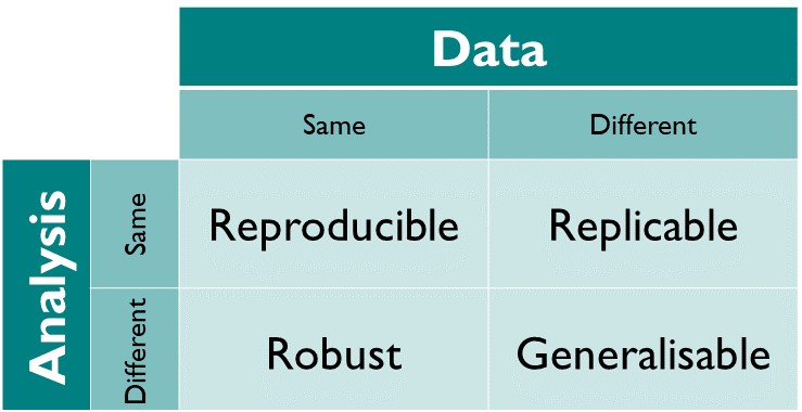
Fig. 1.2 How the Turing Way defines reproducible research [Community et al., 2022] (maybe redraw later).
The Turing Way defines reproducible research as work that can be independently recreated from the same data and the same code that the original team used. The different dimensions of reproducible research in the figure above are further defined as:
Reproducible: A result is reproducible when the same analysis steps performed on the same dataset consistently produces the same answer.
Replicable: A result is replicable when the same analysis performed on different datasets produces qualitatively similar answers.
Robust: A result is robust when the same dataset is subjected to different analysis workflows to answer the same research question (for example one pipeline written in R and another written in Python) and a qualitatively similar or identical answer is produced. Robust results show that the work is not dependent on the specificities of the programming language chosen to perform the analysis.
Generalisable: Combining replicable and robust findings allow us to form generalisable results. Note that running an analysis on a different software implementation and with a different dataset does not provide generalised results. There will be many more steps to know how well the work applies to all the different aspects of the research question. Generalisation is an important step towards understanding that the result is not dependent on a particular dataset nor a particular version of the analysis pipeline.
From the above, we can see that reproducibility is a minimal requirement for reproducible research.
1.2.5. Exercises
1. What are the main ingredients of an ML system?
Compare your answer with the solution below
data, model, and loss function
2. Weight and biases are the hyperparameters of a model.
   a. True

   b. False
Compare your answer with the solution below
b. False. Weight and biases are the parameters of a model. Hyperparameters are the high-level parameters of a model that typically need to be specified before learning a model.
3. Which of the following are true?
   a. In regression, the loss function measures the difference between the predicted class label and the true class label.

   b. In dimensionality reduction, the loss function measures the difference between the predicted real number and the true real number.

   c. In clustering, the loss function measures the coherence and separation of clusters.

   d. In classification, the loss function measures the difference between the predicted class label and the true class label.
Compare your answer with the solution below
c, d
4. Pricing apartments based on a real estate website. We have thousands of house descriptions with their price. Typically, an example of a house description is the following:
Great for entertaining, spacious, updated two bedroom, one bathroom apartment in Lakeview. The house will be available from May 1st. Close to nightlife with a private backyard. Price \(1,000,000\$\).
We are interested in predicting house prices from their description. One potential use case for this would be, as a buyer, finding cheap houses compared to their market value.
4.1. What kind of problem is it? You can choose multiple answers.
 a. a supervised learning problem

 b. an unsupervised learning problem

 c. a classification problem

 d. a regression problem

 e. a clustering problem

 f. a dimensionality reduction problem
Compare your answer with the solution below
a, d. As the label is known, so it is a supervised problem, and then we are trying to predict a continuous value which means it is a regression problem.
4.2. What are the features? You can choose multiple answers.
 a. the number of rooms might be a feature

 b. the postcode of the house might be a feature

 c. the price of the house might be a feature
Compare your answer with the solution below
a, b
4.3. What is the target variable? You have to choose a single answer.
 a. the full-text description is the target

 b. the price of the house is the target

 c. only house descriptions with no price mentioned are the target
Compare your answer with the solution below
b
4.4. What is a record/sample? You have to choose a single answer.
 a. each house description is a record/sample

 b. each house price is a record/sample

 c. each attribute/features of description (as the house size) is a record/sample.
Compare your answer with the solution below
a