K-means and hierarchical clustering
Contents
9.2. \(K\)-means and hierarchical clustering
Clustering, or cluster analysis, refers to methods for finding subgroups, or clusters, in a dataset. When we cluster the observations (data samples) of a dataset, we seek to partition them into distinct groups so that the observations within each group are quite similar to each other, while observations in different groups are quite different from each other. Typically, similarity between observations is defined as the Euclidean distance between their features.
Both clustering and PCA seek to simplify the data via a small number of summaries, but their mechanisms are different:
PCA looks to find a lower-dimensional representation of the observations that explain a good proportion of the variance;
Clustering looks to find homogeneous subgroups among the observations.
Recall Table 1.1, PCA and clustering can be viewed as regression and classification problems under the unsupervised learning paradigm, respectively. PCA outputs a set of numerical values (lower-dimensional feature), while clustering outputs a set of labels (cluster indices).
There are many clustering methods. In this section, we focus on two popular clustering approaches: \(K\)-means clustering and hierarchical clustering. In \(K\)-means clustering, we seek to partition the observations into a pre-specified number of clusters. On the other hand, in hierarchical clustering, we do not know in advance how many clusters we want so we produce a tree-like visual representation of the observations, called a dendrogram, allowing us to view at once the clusterings obtained for each possible number of clusters, from \(1\) to \(N\).
While we focus on clustering observations on the basis of the features in order to identify subgroups among the observations, we can also cluster features on the basis of the observations in order to discover subgroups among the features, e.g. by simply transposing the data matrix.
9.2.1. \(K\)-means clustering
\(K\)-means clustering is a simple and elegant approach for partitioning a dataset into \(K\) distinct, non-overlapping clusters, each represented by its cluster centre (centroid). To perform \(K\)-means clustering, we must first specify the desired number of clusters \(K\); then the \(K\)-means algorithm will assign each observation to exactly one of the \(K\) clusters.
Watch the 8-minute video below for a visual explanation of \(K\)-means clustering.
Video
Explaining \(K\)-Means Clustering by StatQuest, embedded according to YouTube’s Terms of Service.
9.2.1.1. \(K\)-means objective function
The \(K\)-means clustering procedure results from a simple and intuitive mathematical problem. We begin by defining some notation. Let \(C_1, \ldots, C_K\) denote sets containing the indices of the observations in each cluster. These sets satisfy two properties:
\(C_1 \cup C_2 \cup \ldots \cup C_K = {1, \ldots , N} \). In other words, each observation belongs to at least one of the \(K\) clusters.
\(C_k \cap C_{k^′} = \Phi \text{ for all } k \neq k^′\). In other words, the clusters are non-overlapping: no observation belongs to more than one cluster.
For instance, if the \(n\)th observation is in the \(k\text{th}\) cluster, then \(n \in C_k \). The idea behind \(K\)-means clustering is that a good clustering is one for which the within-cluster variation is as small as possible. The within-cluster variation for cluster \(C_k\) is a measure \(W(C_k)\) of the amount by which the observations within a cluster differ from each other, a concept similar to variation studied in PCA. Hence we want to solve the problem
In words, this formula says that we want to partition the observations into \(K\) clusters such that the total within-cluster variation, summed over all \(K\) clusters, is as small as possible.
In order to make solving Equation (9.3) actionable we need to define the within-cluster variation. There are many possible ways to define this concept, but by far the most common choice involves squared Euclidean distance. That is, we define
where \(|C_k|\) denotes the number of observations in the \(k\text{th}\) cluster. In other words, the within-cluster variation for the \(k\)th cluster is the sum of all of the pairwise squared Euclidean distances between the observations in the \(k\text{th}\) cluster, divided by the total number of observations in the \(k\text{th}\) cluster.
Combining Equations (9.3) and (9.4), gives the optimization problem that defines \(K\)-means clustering,
9.2.1.2. \(K\)-means algorithm
Now, we would like to find an algorithm to solve Equation (9.5)—that is, a method to partition the observations into \(K\) clusters such that the objective of Equation (9.5) is minimised. This is in fact a very difficult problem to solve precisely, since there are almost \(K^N\) ways to partition \(N\) observations into \(K\) clusters. This is a huge number unless \(K\) and \(N\) are tiny! Fortunately, a very simple algorithm can be shown to provide a local optimum, i.e. a pretty good (but not necessarily the best) solution, to the \(K\)-means optimisation problem (9.5). This approach is laid out in Algorithm 9.1.
Algorithm 9.1 (\(K\)-means Clustering)
Randomly assign a number, from \(1\) to \(K\), to each of the observations. These serve as initial cluster assignments for the observations.
Iterate until the cluster assignments stop changing:
(a) For each of the \(K\) clusters, compute the cluster centroid, which is the vector of the \(D\) feature means of the observations in the \(k\text{th}\) cluster.
(b) Assign each observation to the cluster for which the squared Euclidean distance between the observation and the cluster centroid is smallest.
Algorithm 9.1 is guaranteed to decrease the value of the objective (9.5) at each step. To understand why, the following identity is illuminating:
where \(\bar{x}_{k,d}\) is the mean of the \(d\text{th}\) feature for the observations in the \(k\text{th}\) cluster. In Step 2(a) of Algorithm 9.1, the cluster means for each feature are the constants that minimise the sum-of-squared deviations. In Step 2(b), reallocating the observations can only improve Equation (9.6). This means that as the algorithm is run, the clustering obtained will continually improve until the result no longer changes; the objective of Equation (9.5) will never increase. When the result no longer changes, a local optimum has been reached.
Because the \(K\)-means algorithm finds a local rather than a global optimum, the results obtained will depend on the initial (random) cluster assignment of each observation in Step 1 of Algorithm 9.1. For this reason, it is important to run the algorithm multiple times from different random initial configurations and to set a random seed for reproducibility. Then one selects the best solution, i.e. that for which the objective in Eq. (9.5) is the smallest.
9.2.1.3. \(K\)-means clustering on toy data with scikit-learn
Get ready by importing the APIs needed from respective libraries.
import pandas as pd
import numpy as np
from numpy.linalg import svd
import matplotlib as mpl
import matplotlib.pyplot as plt

from sklearn.preprocessing import StandardScaler
from sklearn.decomposition import PCA
from sklearn.cluster import KMeans
from scipy.cluster import hierarchy

%matplotlib inline
Generate some toy data to study the \(K\)-means algorithm. Set a random seed for reproducibility.
np.random.seed(21)
X = np.random.standard_normal((50, 2))
X[:25, 0] = X[:25, 0] + 3
X[:25, 1] = X[:25, 1] - 4
Fit \(K\)-means models with \(K=2\) and \(3\), respectively:
n_clusters = 2
km1 = KMeans(n_clusters=n_clusters, n_init=20)
km1.fit(X)

n_clusters = 3
km2 = KMeans(n_clusters=n_clusters, n_init=20)
km2.fit(X)
KMeans(n_clusters=3, n_init=20)In a Jupyter environment, please rerun this cell to show the HTML representation or trust the notebook.
On GitHub, the HTML representation is unable to render, please try loading this page with nbviewer.org.
KMeans(n_clusters=3, n_init=20)
Inspect the first \(K\)-means model:
print(km1.labels_)
print(dir(km1))  # we can use dir to see other saved attributes
[0 0 0 0 0 0 0 0 0 0 0 0 0 0 0 0 0 0 0 0 0 0 0 0 0 1 1 1 1 1 1 1 1 1 1 1 1
 1 1 1 1 1 1 1 1 1 1 1 1 1]
['__abstractmethods__', '__annotations__', '__class__', '__delattr__', '__dict__', '__dir__', '__doc__', '__eq__', '__format__', '__ge__', '__getattribute__', '__getstate__', '__gt__', '__hash__', '__init__', '__init_subclass__', '__le__', '__lt__', '__module__', '__ne__', '__new__', '__reduce__', '__reduce_ex__', '__repr__', '__setattr__', '__setstate__', '__sizeof__', '__sklearn_clone__', '__slots__', '__str__', '__subclasshook__', '__weakref__', '_abc_impl', '_algorithm', '_build_request_for_signature', '_check_feature_names', '_check_mkl_vcomp', '_check_n_features', '_check_params_vs_input', '_check_test_data', '_estimator_type', '_get_default_requests', '_get_metadata_request', '_get_param_names', '_get_tags', '_init_centroids', '_more_tags', '_n_features_out', '_n_init', '_n_threads', '_parameter_constraints', '_repr_html_', '_repr_html_inner', '_repr_mimebundle_', '_sklearn_auto_wrap_output_keys', '_tol', '_transform', '_validate_center_shape', '_validate_data', '_validate_params', '_warn_mkl_vcomp', 'algorithm', 'cluster_centers_', 'copy_x', 'fit', 'fit_predict', 'fit_transform', 'get_feature_names_out', 'get_metadata_routing', 'get_params', 'inertia_', 'init', 'labels_', 'max_iter', 'n_clusters', 'n_features_in_', 'n_init', 'n_iter_', 'predict', 'random_state', 'score', 'set_fit_request', 'set_output', 'set_params', 'set_predict_request', 'set_score_request', 'tol', 'transform', 'verbose']
We can see the cluster assignments for each observation.
Let us plot a figure that shows the results obtained from performing \(K\)-means clustering on the simulated examples, using two different values of \(K\).
fig, (ax1, ax2) = plt.subplots(1, 2, figsize=(14, 5))

ax1.scatter(X[:, 0], X[:, 1], s=40, c=km1.labels_, cmap=plt.cm.prism)
ax1.set_title("$K$-means Clustering Results with $K$=2")
ax1.scatter(
    km1.cluster_centers_[:, 0],
    km1.cluster_centers_[:, 1],
    marker="+",
    s=100,
    c="k",
    linewidth=2,
)

ax1.scatter(
    X[1, 0],
    X[1, 1],
    alpha=0.8,
    facecolors="none",
    marker="o",
    edgecolors="blue",
    linewidths=3,
)

ax2.scatter(X[:, 0], X[:, 1], s=40, c=km2.labels_, cmap=plt.cm.prism)
ax2.set_title("$K$-means Clustering Results with $K$=3")
ax2.scatter(
    km2.cluster_centers_[:, 0],
    km2.cluster_centers_[:, 1],
    marker="+",
    s=100,
    c="k",
    linewidth=2,
)


plt.show()
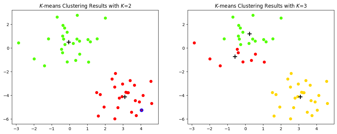
Let us examine a particular data point to explain the system transparency of \(K\)-means clustering.
print("Data sample point : \n", np.around(X[1], 2))

print("Centre coordinates for K=2: \n", np.around(km1.cluster_centers_, 2))

print(
    "Distance of sample point from each cluster centre: \n",
    np.around(km1.transform(X[1].reshape(1, -1))[0], 2),
)
Data sample point :
 [ 4.04 -5.26]
Centre coordinates for K=2:
 [[ 3.09 -4.12]
 [-0.06  0.51]]
Distance of sample point from each cluster centre:
 [1.48 7.08]
System transparency
When \(K=2\), the centres of the two clusters are \([ 3.09 \;\; -4.12]\) (red cluster) and \([-0.06 \;\; 0.51]\) (green cluster). For the data point \( [4.04 \;\; -5.26]^{\top} \), its distance to the red cluster centre is \(1.48\) and to the green cluster centre is \(7.08\). Hence, it is assigned to the red cluster.
When \(K=2\), given a particular cluster \(k\), e.g. the green cluster centred at \([-0.06 \;\; 0.51]\), any data point \([x_1, x_2]\) belong to this cluster should satisfy the following condition:
Note: numbers are limited to two decimal places for the sake of clarity.
9.2.2. Hierarchical clustering
One potential disadvantage of \(K\)-means clustering is that it requires us to pre-specify the number of clusters \(K\), which will need to employ a model selection (hyperparameter tuning) method. Hierarchical clustering is an alternative approach which does not require that we commit to a particular choice of \(K\). Hierarchical clustering has an added advantage over \(K\)-means clustering in that it results in an attractive tree-based representation of the observations, called a dendrogram.
9.2.2.1. Hierarchical clustering on toy data
Using the same toy data above, let us plot a figure to demonstrate bottom-up or agglomerative clustering. This is the most common type of hierarchical clustering, and refers to the fact that a dendrogram (generally depicted as an upside-down tree) is built starting from the leaves and combining clusters up to the trunk.
fig, (ax1, ax2, ax3) = plt.subplots(3, 1, figsize=(15, 18))

for linkage, cluster, ax in zip(
    [hierarchy.complete(X), hierarchy.average(X), hierarchy.single(X)],
    ["c1", "c2", "c3"],
    [ax1, ax2, ax3],
):
    cluster = hierarchy.dendrogram(linkage, ax=ax, color_threshold=0)

ax1.set_title("Complete Linkage")
ax2.set_title("Average Linkage")
ax3.set_title("Single Linkage")
plt.show()
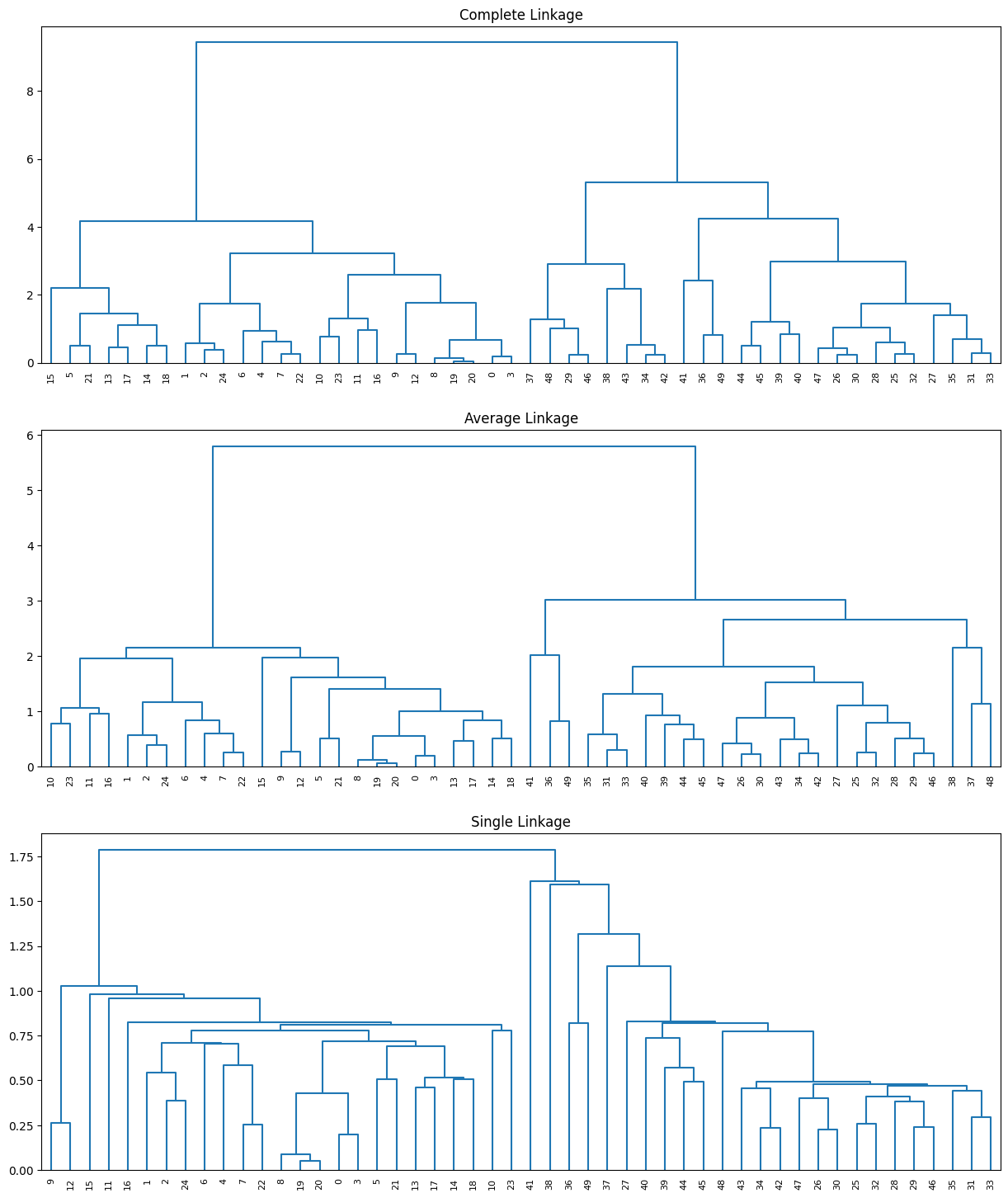
In the top panel of the figure above, each leaf (at the bottom) of the dendrogram represents one of the 50 toy examples generated previously. However, as we move up the tree, some leaves begin to fuse into branches. These correspond to observations that are similar to each other. As we move higher up the tree, branches themselves fuse, either with leaves or other branches. The earlier (lower in the tree) fusions occur, the more similar the groups of observations are to each other. On the other hand, observations that fuse later (near the top of the tree) can be quite different. In fact, this statement can be made precise: for any two observations, we can look for the point in the tree where branches containing those two observations are first fused. The height of this fusion, as measured on the vertical axis, indicates how different the two observations are. Thus, observations that fuse at the very bottom of the tree are quite similar to each other, whereas observations that fuse close to the top of the tree will tend to be quite different.
9.2.2.2. The hierarchical clustering Algorithm
The hierarchical clustering dendrogram is obtained via an extremely simple algorithm. We begin by defining some sort of dissimilarity measure between each pair of observations. Most often, Euclidean distance is used. The algorithm proceeds iteratively. Starting out at the bottom of the dendrogram, each of the \(N\) observations is treated as its own cluster. The two clusters that are most similar to each other are then fused so that there are \(N\) − 1 clusters after this first fusion. Next the two clusters that are most similar to each other are fused again, so that there are \(N\) − 2 clusters after the second fusion. The algorithm proceeds in this fashion until all of the observations belong to one single cluster, and the dendrogram is complete. Algorithm 9.2 summarises the hierarchical clustering algorithm.
Algorithm 9.2 (Hierarchical clustering)
Begin with \(N\) observations and a measure (such as Euclidean distance) of all the \(N(N − 1)/2\) pairwise dissimilarities. Treat each observation as its own cluster.
For \(n = N, N − 1, \ldots, 2\):
(a) Examine all pairwise inter-cluster dissimilarities among the \(n\) clusters and identify the pair of clusters that are least dissimilar (that is, most similar). Fuse these two clusters. The dissimilarity between these two clusters indicates the height in the dendrogram at which the fusion should be placed.
(b) Compute the new pairwise inter-cluster dissimilarities among the \(n − 1\) remaining clusters.
We have a concept of the dissimilarity between pairs of observations, but how do we define the dissimilarity between two clusters if one or both of the clusters contains multiple observations? The concept of dissimilarity between a pair of observations needs to be extended to a pair of groups of observations. This extension is achieved by developing the notion of linkage, which defines the dissimilarity between two groups of observations. The four most common types of linkage—complete, average, single, and centroid. Table 9.1 summarises the four types of linkage.
The figure generated in the code cell above shows the clustering results of average, complete, and single linkage on the toy dataset, where we can observe that average and complete linkage methods tend to yield more balanced clusters (trees).
Linkage |
Description |
|---|---|
Complete |
Maximal inter-cluster dissimilarity. Compute all pairwise dissimilarities between the observations in cluster A and the observations in cluster B, and record the largest of these dissimilarities. |
Single |
Minimal inter-cluster dissimilarity. Compute all pairwise dissimilarities between the observations in cluster A and the observations in cluster B, and record the smallest of these dissimilarities. Single linkage can result in extended, trailing clusters in which single observations are fused one-at-a-time. |
Average |
Mean inter-cluster dissimilarity. Compute all pairwise dissimilarities between the observations in cluster A and the observations in cluster B, and record the average of these dissimilarities. |
Centroid |
Dissimilarity between the centroid for cluster A (a mean vector of length \(D\)) and the centroid for cluster B. Centroid linkage can result in undesirable inversions. |
9.2.2.3. Hierarchical clustering to explore cancer cell line microarray data
We illustrate these hierarchical clustering on the NCI60 cancer cell line microarray data, which consists of 6,830 gene expression measurements on 64 cancer cell lines.
Load the data and inspect the first few rows of the data frame.
X = pd.read_csv("https://github.com/pykale/transparentML/raw/main/data/NCI60_data.csv")
y = pd.read_csv("https://github.com/pykale/transparentML/raw/main/data/NCI60_labs.csv")

y.head()
| x | |
|---|---|
| 0 | CNS |
| 1 | CNS |
| 2 | CNS |
| 3 | RENAL |
| 4 | BREAST |
Each cell line is labelled with a cancer type, given in y. We do not make use of the cancer types in performing clustering since we are studying unsupervised learning here. After performing clustering, we will check to see the extent to which these cancer types agree with the clustering results.
Inspect the data size.
X.shape
(64, 6830)
The data has 64 rows and 6,830 columns.
Standardise the data.
scaler = StandardScaler()
X_scaled = pd.DataFrame(scaler.fit_transform(X), index=y.iloc[:, 0], columns=X.columns)
We now perform hierarchical clustering of the observations using complete, single, and average linkage. Euclidean distance is used as the dissimilarity measure.
fig, (ax1, ax2, ax3) = plt.subplots(1, 3, figsize=(20, 20))

for linkage, cluster, ax in zip(
    [hierarchy.complete(X_scaled), hierarchy.average(X), hierarchy.single(X_scaled)],
    ["c1", "c2", "c3"],
    [ax1, ax2, ax3],
):
    cluster = hierarchy.dendrogram(
        linkage,
        labels=X_scaled.index,
        orientation="right",
        color_threshold=0,
        leaf_font_size=10,
        ax=ax,
    )

ax1.set_title("Complete Linkage")
ax2.set_title("Average Linkage")
ax3.set_title("Single Linkage")
plt.show()
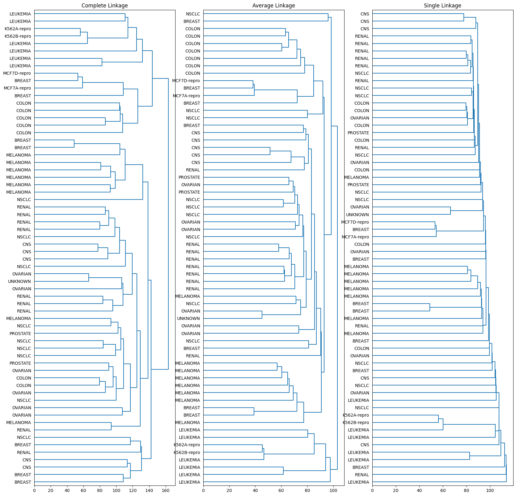
We can see the above for the NCI60 cancer cell line microarray data clustered with average, complete, and single linkage, using Euclidean distance as the dissimilarity measure. As earlier, complete and average linkage tend to yield evenly sized clusters whereas single linkage tends to yield extended clusters to which single leaves are fused one by one.
After obtain the dendrogram, we can take a cut at the desired height to obtain a partition of the observations into \(K\) clusters.
plt.figure(figsize=(10, 20))
cut4 = hierarchy.dendrogram(
    hierarchy.complete(X_scaled),
    labels=X_scaled.index,
    orientation="right",
    color_threshold=140,
    leaf_font_size=10,
)
plt.vlines(
    140, 0, plt.gca().yaxis.get_data_interval()[1], colors="r", linestyles="dashed"
)
plt.show()
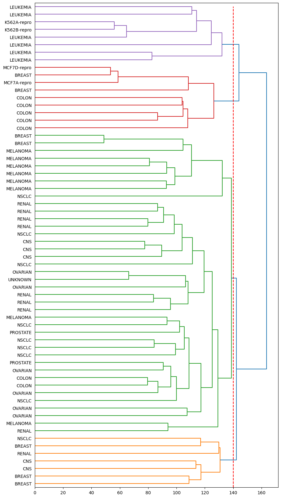
Here, we take a cut at a height of 140 to obtain four clusters.
9.2.3. Exercises
1. In this exercise, you will generate your own simulated data and perform PCA and \(K\)-means clustering.
(a) Generate a simulated 50-dimensional dataset consisting of 3 classes, with each class containing \(20\) observations. Your dataset should have a shape of [60, 50], i.e \(60\) observations in total, nad each with \(50\) variables. Think carefully about how you can define your 3 classes. For example, you could use the np.random.normal() function to create your 3 classes, changing the mean and standard deviation of each class using the loc & scale parameters!
# Write your code below to answer the question
Compare your answer with the reference solution below
import numpy as np

## Generate the data
true_cluster_1 = np.random.normal(loc=-5, scale=0.5, size=(20, 50))
true_cluster_2 = np.random.normal(loc=10, scale=1, size=(20, 50))
true_cluster_3 = np.random.normal(loc=5, scale=0.9, size=(20, 50))

## Combine the data into a single array
combined = np.append(
    true_cluster_1, np.append(true_cluster_2, true_cluster_3, axis=0), axis=0
)
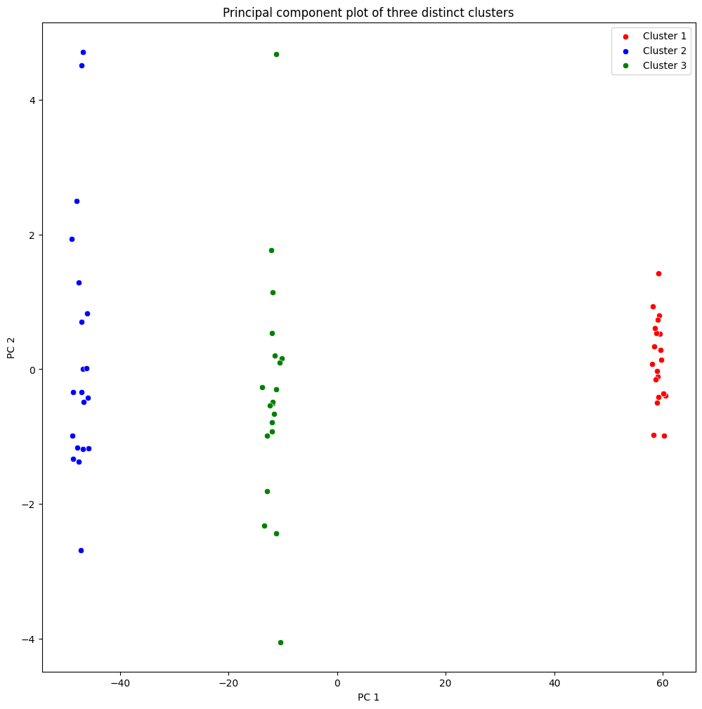
(b) Perform PCA on the \(60\) observations and plot the first two principal component score vectors. Use a different colour to indicate the observations in each of the three classes. If the three classes appear separated in this plot, then continue on to part (c). If not, then return to part (a) and modify the simulation so that there is greater separation between the three classes. Do not continue to part (c) until the three classes show at least some separation in the first two principal component score vectors.
# Write your code below to answer the question
Compare your answer with the reference solution below
import matplotlib.pyplot as plt
import seaborn as sns
from sklearn.decomposition import PCA

## Break the data into Principal components
pca = PCA(n_components=2)
pca.fit(combined)

X = pca.transform(combined)

fig, ax1 = plt.subplots(nrows=1, ncols=1, figsize=(12, 12))
sns.scatterplot(x=X[0:20, 0], y=X[0:20, 1], color="r", label="Cluster 1")
sns.scatterplot(x=X[20:40, 0], y=X[20:40, 1], color="b", label="Cluster 2")
sns.scatterplot(x=X[40:60, 0], y=X[40:60, 1], color="g", label="Cluster 3")

ax1.set_xlabel("PC 1")
ax1.set_ylabel("PC 2")

ax1.set_title("Principal component plot of three distinct clusters")

ax1.legend()
plt.show()
(c) Perform \(K\)-means clustering of the observations with \(K = 3\). How well do the clusters that you obtained in \(K\)-means clustering compare to the true class labels?
# Write your code below to answer the question
Compare your answer with the reference solution below
from sklearn.cluster import KMeans

np.random.seed(2022)
## Break the data into Principal components
kmeans = KMeans(n_clusters=3, n_init=10)

X = kmeans.fit_predict(combined)
print("True Cluster 1 predictions:")
print(X[0:20])
print("True Cluster 2 predictions:")
print(X[20:40])
print("True Cluster 3 predictions:")
print(X[40:60])

# We see that there is perfect recall of the true clusters. We can not produce a nice plot as in part b) as it is 50 dimensional.
True Cluster 1 predictions:
[0 0 0 0 0 0 0 0 0 0 0 0 0 0 0 0 0 0 0 0]
True Cluster 2 predictions:
[1 1 1 1 1 1 1 1 1 1 1 1 1 1 1 1 1 1 1 1]
True Cluster 3 predictions:
[2 2 2 2 2 2 2 2 2 2 2 2 2 2 2 2 2 2 2 2]
(d) Perform \(K\)-means clustering with \(K = 2\). Describe your results.
# Write your code below to answer the question
Compare your answer with the reference solution below
## Break the data into Principal components
np.random.seed(2022)
kmeans = KMeans(n_clusters=2)

X = kmeans.fit_predict(combined)
print("True Cluster 1 predictions:")
print(X[0:20])
print("True Cluster 2 predictions:")
print(X[20:40])
print("True Cluster 3 predictions:")
print(X[40:60])

# Here it has clustered the last two clusters into one.
# This seems intuitive looking at the PCA plot as these two clusters are the most similar on the first two PCs
True Cluster 1 predictions:
[0 0 0 0 0 0 0 0 0 0 0 0 0 0 0 0 0 0 0 0]
True Cluster 2 predictions:
[1 1 1 1 1 1 1 1 1 1 1 1 1 1 1 1 1 1 1 1]
True Cluster 3 predictions:
[1 1 1 1 1 1 1 1 1 1 1 1 1 1 1 1 1 1 1 1]
/opt/hostedtoolcache/Python/3.8.18/x64/lib/python3.8/site-packages/sklearn/cluster/_kmeans.py:1416: FutureWarning: The default value of `n_init` will change from 10 to 'auto' in 1.4. Set the value of `n_init` explicitly to suppress the warning
  super()._check_params_vs_input(X, default_n_init=10)
(d) Now perform \(K\)-means clustering with \(K = 4\) , and describe your results.
# Write your code below to answer the question
Compare your answer with the reference solution below
## Break the data into Principal components
np.random.seed(2022)

kmeans = KMeans(n_clusters=4)

X = kmeans.fit_predict(combined)
print("True Cluster 1 prdictions:")
print(X[0:20])
print("True Cluster 2 prdictions:")
print(X[20:40])
print("True Cluster 3 prdictions:")
print(X[40:60])

# Setting the number of desired clusters as more than the true number means that at least one will have to split up.
# In this example, setting n=4 makes the second cluster split into two. This is because it has the most variance compared to the other two clusters.
True Cluster 1 prdictions:
[1 1 1 1 1 1 1 1 1 1 1 1 1 1 1 1 1 1 1 1]
True Cluster 2 prdictions:
[0 0 0 3 0 0 3 0 0 3 0 0 3 0 0 3 0 0 0 0]
True Cluster 3 prdictions:
[2 2 2 2 2 2 2 2 2 2 2 2 2 2 2 2 2 2 2 2]
/opt/hostedtoolcache/Python/3.8.18/x64/lib/python3.8/site-packages/sklearn/cluster/_kmeans.py:1416: FutureWarning: The default value of `n_init` will change from 10 to 'auto' in 1.4. Set the value of `n_init` explicitly to suppress the warning
  super()._check_params_vs_input(X, default_n_init=10)
(e) Using the StandardScaler function, perform \(K\)-means clustering with \(K = 3\) on the data after scaling each variable to have a standard deviation of one.
# Write your code below to answer the question
Compare your answer with the reference solution below
## Break the data into Principal components
from sklearn.preprocessing import StandardScaler

np.random.seed(2022)

scaler = StandardScaler(with_mean=False)
scaler.fit(combined)
data = scaler.transform(combined)

kmeans = KMeans(n_clusters=3, n_init=10)

X = kmeans.fit_predict(combined)
print("True Cluster 1 prdictions:")
print(X[0:20])
print("True Cluster 2 prdictions:")
print(X[20:40])
print("True Cluster 3 prdictions:")
print(X[40:60])
True Cluster 1 prdictions:
[0 0 0 0 0 0 0 0 0 0 0 0 0 0 0 0 0 0 0 0]
True Cluster 2 prdictions:
[1 1 1 1 1 1 1 1 1 1 1 1 1 1 1 1 1 1 1 1]
True Cluster 3 prdictions:
[2 2 2 2 2 2 2 2 2 2 2 2 2 2 2 2 2 2 2 2]
2. Consider the USArrests dataset. We will now perform hierarchical clustering on the states.
(a) Load the USArrests dataset, rename the index of each row to its corresponding state name and finally drop the column of state names from the original data frame.
# Write your code below to answer the question
Compare your answer with the reference solution below
import pandas as pd
from sklearn.preprocessing import StandardScaler


USArrests = pd.read_csv(
    "https://github.com/pykale/transparentML/raw/main/data/USArrests.csv"
)

state_name = USArrests.iloc[:, 0]  # abstract a list of state names

# rename index of each row to its corresponding state name
USArrests = USArrests.rename(index=lambda x: state_name[x])

# drop the column of state name from the original data frame
USArrests.drop(USArrests.columns[[0]], axis=1, inplace=True)
scaled_x = StandardScaler().fit_transform(USArrests)
(b) Using agglomerative hierarchical clustering with complete linkage and Euclidean distance, cluster the states.
# Write your code below to answer the question
Compare your answer with the reference solution below
from scipy.cluster.hierarchy import linkage

hc_complete1 = linkage(USArrests, "complete")
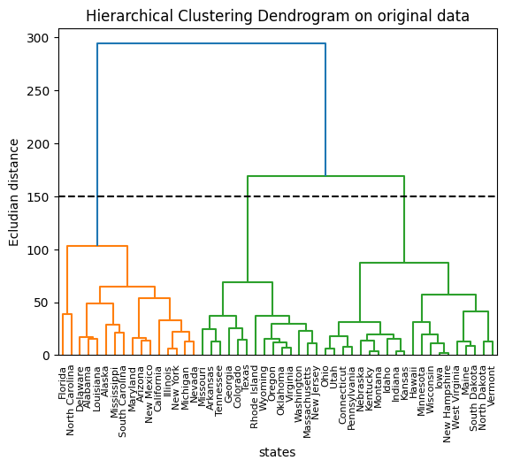
(c) Cut the dendrogram at a height that results in three distinct clusters. Which states belong to which clusters?
# Write your code below to answer the question
Compare your answer with the reference solution below
from scipy.cluster.hierarchy import dendrogram, cut_tree
import matplotlib.pyplot as plt

res1 = pd.DataFrame(cut_tree(hc_complete1, n_clusters=3), index=state_name)
res1.index.name = "states"
res1.rename(columns={0: "Clusters"}, inplace=True)

# dendrogram
plt.figure(2)
plt.title("Hierarchical Clustering Dendrogram on original data")
plt.xlabel("states")
plt.ylabel("Ecludian distance")
dendrogram(hc_complete1, labels=res1.index, leaf_rotation=90, leaf_font_size=8)
plt.axhline(y=150, c="k", ls="dashed")
plt.show()

print(res1)

# Cutting the dendrogram at height 150 results in three distinct clusters.
                Clusters
states
Alabama                0
Alaska                 0
Arizona                0
Arkansas               1
California             0
Colorado               1
Connecticut            2
Delaware               0
Florida                0
Georgia                1
Hawaii                 2
Idaho                  2
Illinois               0
Indiana                2
Iowa                   2
Kansas                 2
Kentucky               2
Louisiana              0
Maine                  2
Maryland               0
Massachusetts          1
Michigan               0
Minnesota              2
Mississippi            0
Missouri               1
Montana                2
Nebraska               2
Nevada                 0
New Hampshire          2
New Jersey             1
New Mexico             0
New York               0
North Carolina         0
North Dakota           2
Ohio                   2
Oklahoma               1
Oregon                 1
Pennsylvania           2
Rhode Island           1
South Carolina         0
South Dakota           2
Tennessee              1
Texas                  1
Utah                   2
Vermont                2
Virginia               1
Washington             1
West Virginia          2
Wisconsin              2
Wyoming                1
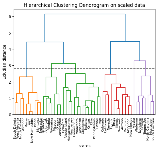
(d) Perform agglomerative hierarchical clustering of the states using complete linkage and Euclidean distance after scaling the variables to have a standard deviation of one. Then, cut the dendrogram at a height that results in six distinct clusters. Which states belong to which clusters?
# Write your code below to answer the question
Compare your answer with the reference solution below
hc_complete2 = linkage(scaled_x, "complete")
res2 = pd.DataFrame(cut_tree(hc_complete2, n_clusters=6), index=state_name)
res2.index.name = "states"
res2.rename(columns={0: "ID"}, inplace=True)

plt.figure(3)
plt.title("Hierarchical Clustering Dendrogram on scaled data")
plt.xlabel("states")
plt.ylabel("Ecludian distance")
dendrogram(hc_complete2, labels=res2.index, leaf_rotation=90, leaf_font_size=8)
plt.axhline(y=2.8, c="k", ls="dashed")
plt.show()

print(res2)
# Cutting the dendrogram at height 2.8 results in six distinct clusters.
                ID
states
Alabama          0
Alaska           1
Arizona          2
Arkansas         3
California       2
Colorado         2
Connecticut      4
Delaware         4
Florida          2
Georgia          0
Hawaii           4
Idaho            5
Illinois         2
Indiana          4
Iowa             5
Kansas           4
Kentucky         3
Louisiana        0
Maine            5
Maryland         2
Massachusetts    4
Michigan         2
Minnesota        4
Mississippi      0
Missouri         3
Montana          5
Nebraska         5
Nevada           2
New Hampshire    5
New Jersey       4
New Mexico       2
New York         2
North Carolina   0
North Dakota     5
Ohio             4
Oklahoma         4
Oregon           3
Pennsylvania     4
Rhode Island     4
South Carolina   0
South Dakota     5
Tennessee        0
Texas            2
Utah             4
Vermont          5
Virginia         3
Washington       3
West Virginia    5
Wisconsin        4
Wyoming          3