.ipynb .pdf

repository open issue suggest edit

Binder Colab

Contents

5.2. Bootstrap

From the previous section, we have seen that it is common to encounter randomness in performance evaluation. Even with cross-validation, such randomness can still be present. In this case, it will be good to have an estimation of the uncertainty of the performance metric obtained. This is where the bootstrap, or bootstrapping comes in.

The bootstrap is a widely applicable and extremely powerful resampling method that can be used to quantify the uncertainty associated with a performance metric for machine learning models. It is a non-parametric method, meaning that it does not make any assumptions about the underlying distribution of the data. It is also a model-free method, meaning that it does not require a model to be fit to the data.

The bootstrap is a general technique for estimating the sampling distribution of a statistic by sampling from the data with replacement. The bootstrap can be used to estimate the sampling distribution of ANY statistic, including the mean, standard deviation, correlation coefficient, and regression coefficients. The bootstrap can also be used to estimate the sampling distribution of a machine learning model, such as the coefficients of a linear regression model.

As a simple example, the bootstrap can be used to estimate the standard errors of the coefficients from a linear regression fit. Although standard errors were obtained automatically by statsmodels in Linear regression and Logistic regression, the power of the bootstrap lies in the fact that it can be easily applied to a wide range of machine learning models.

Watch the 6-minute video below for a visual explanation of cross-validation:

Video

Explaining Cross Bootstrap by StatQuest, embedded according to YouTube’s Terms of Service.

5.2.1. Import libraries and load data

Get ready by importing the APIs needed from respective libraries.

import pandas as pd
import numpy as np
import matplotlib.pyplot as plt
import seaborn as sns

from sklearn.linear_model import LinearRegression
from sklearn.metrics import mean_squared_error
from sklearn.preprocessing import PolynomialFeatures
from sklearn.utils import resample

%matplotlib inline

Set a random seed for reproducibility.

np.random.seed(2022)

We use the same Auto dataset as in the previous section.

auto_url = "https://github.com/pykale/transparentML/raw/main/data/Auto.csv"

auto_df = pd.read_csv(auto_url, na_values="?").dropna()
auto_df.info()

<class 'pandas.core.frame.DataFrame'>
Index: 392 entries, 0 to 396
Data columns (total 9 columns):
 #   Column        Non-Null Count  Dtype  
---  ------        --------------  -----  
 0   mpg           392 non-null    float64
 1   cylinders     392 non-null    int64  
 2   displacement  392 non-null    float64
 3   horsepower    392 non-null    float64
 4   weight        392 non-null    int64  
 5   acceleration  392 non-null    float64
 6   year          392 non-null    int64  
 7   origin        392 non-null    int64  
 8   name          392 non-null    object 
dtypes: float64(4), int64(4), object(1)
memory usage: 30.6+ KB

5.2.2. Bootstrap for uncertainty estimation

Suppose that we wish to estimate the uncertainty of a coefficient estimate \(\beta_1\) from a linear regression fit, we take \(M\) (\( M <N \)) repeated samples with replacement from our dataset and train our linear regression model \(B\) times and record each value \(\hat{\beta}_1^{*1}, \hat{\beta}_1^{*2}, \dots, \hat{\beta}_1^{*B}\). With enough resampling, e.g. \(B = 1000\) or \(B = 10,000\), we can plot the distribution of these bootstrapped estimates \(\hat{\beta}_1^{*b}, b = 1,\cdots, B \). Then, we can use the resulting distribution to quantify the variability (or uncertainty, confidence) of this estimate by calculating useful summary statistics, such as standard errors and confidence intervals.

The power of the bootstrap lies in the ability to take repeated samples of the dataset, instead of collecting a new dataset each time. Also, in contrast to standard error estimates typically reported with statistical software that rely on algebraic methods and underlying assumptions (which may be wrong), bootstrapped standard error estimates are more accurate as they are calculated computationally without any pre-specified assumptions.

Let us study the bootstrap on the Auto dataset using the scikit-learn’s resample API (adapted from this blog post).

# Defining number of iterations for bootstrap resample
n_iterations = 1000

# Initializing estimator
lin_reg = LinearRegression()

# Initializing DataFrame, to hold bootstrapped statistics
bootstrapped_stats = pd.DataFrame()

# Each loop iteration is a single bootstrap resample and model fit
for i in range(n_iterations):
    # Sampling n_samples from data, with replacement, as train
    # Defining test to be all observations not in train
    train = resample(auto_df, replace=True, n_samples=len(auto_df))
    test = auto_df[~auto_df.index.isin(train.index)]

    X_train = train.loc[:, ["horsepower", "weight"]]
    y_train = train.loc[:, ["mpg"]]

    X_test = test.loc[:, ["horsepower", "weight"]]
    y_test = test.loc[:, ["mpg"]]

    # Fitting linear regression model
    lin_reg.fit(X_train, y_train)

    # Storing stats in DataFrame, and concatenating with stats
    intercept = lin_reg.intercept_
    beta_horsepower = lin_reg.coef_.ravel()[0]
    beta_weight = lin_reg.coef_.ravel()[1]
    r_squared = lin_reg.score(X_test, y_test)

    bootstrapped_stats_i = pd.DataFrame(
        data=dict(
            intercept=intercept,
            beta_horsepower=beta_horsepower,
            beta_weight=beta_weight,
            r_squared=r_squared,
        )
    )

    bootstrapped_stats = pd.concat(objs=[bootstrapped_stats, bootstrapped_stats_i])

Let us inspect a few estimates.

bootstrapped_stats.head()

	intercept	beta_horsepower	beta_weight	r_squared
0	45.343984	-0.066652	-0.005013	0.702527
0	45.803707	-0.047437	-0.005756	0.702518
0	46.132643	-0.036886	-0.006368	0.708330
0	45.994224	-0.072389	-0.005004	0.709075
0	44.679054	-0.060294	-0.005046	0.723611

Plot the distribution of the bootstrapped estimates of the coefficients and the corresponding test scores for the Auto dataset:

# Plotting histograms
fig, axes = plt.subplots(1, 4, figsize=(18, 5))
sns.histplot(bootstrapped_stats["intercept"], color="royalblue", ax=axes[0], kde=True)
sns.histplot(bootstrapped_stats["beta_horsepower"], color="olive", ax=axes[1], kde=True)
sns.histplot(bootstrapped_stats["beta_weight"], color="gold", ax=axes[2], kde=True)
sns.histplot(bootstrapped_stats["r_squared"], color="teal", ax=axes[3], kde=True)
plt.show()

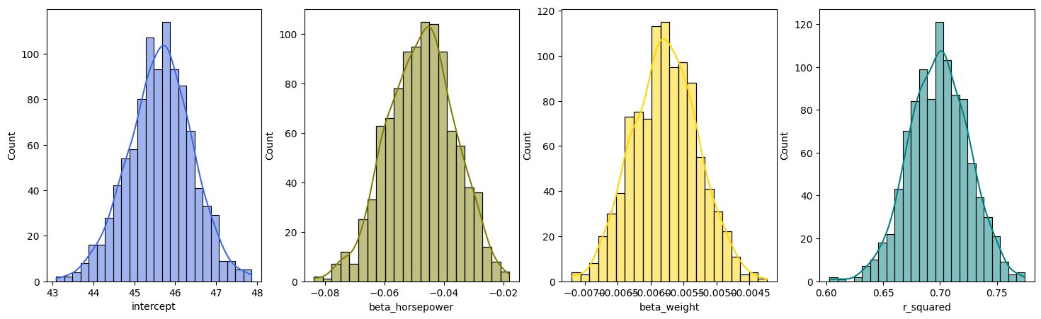
In this way, we can easily estimate the uncertainty of ANY coefficient estimates and ANY test scores.

We can use the resulting distribution to quantify the variability (or uncertainty, confidence) of this estimate by calculating useful summary statistics, such as standard errors and confidence intervals.

First, calculate the mean.

bootstrapped_stats.mean()

intercept          45.628857
beta_horsepower    -0.047742
beta_weight        -0.005776
r_squared           0.698822
dtype: float64

Next, calculate the standard deviation.

bootstrapped_stats.std()

intercept          0.783889
beta_horsepower    0.011256
beta_weight        0.000491
r_squared          0.026071
dtype: float64

Finally, calculate the 95% confidence interval.

bootstrapped_stats.quantile([0.025, 0.975])

	intercept	beta_horsepower	beta_weight	r_squared
0.025	44.011519	-0.070634	-0.006737	0.648188
0.975	47.110089	-0.026996	-0.004826	0.749205

5.2.3. Exercises

1.Bootstrap is a powerfull resmapling method.

   a. True

   b. False

Compare your answer with the solution below

a. True

2. Bootstrap is a parametric method.

   a. True

   b. False

Compare your answer with the solution below

b. False. Bootstrap is a non-parametric model-free method.

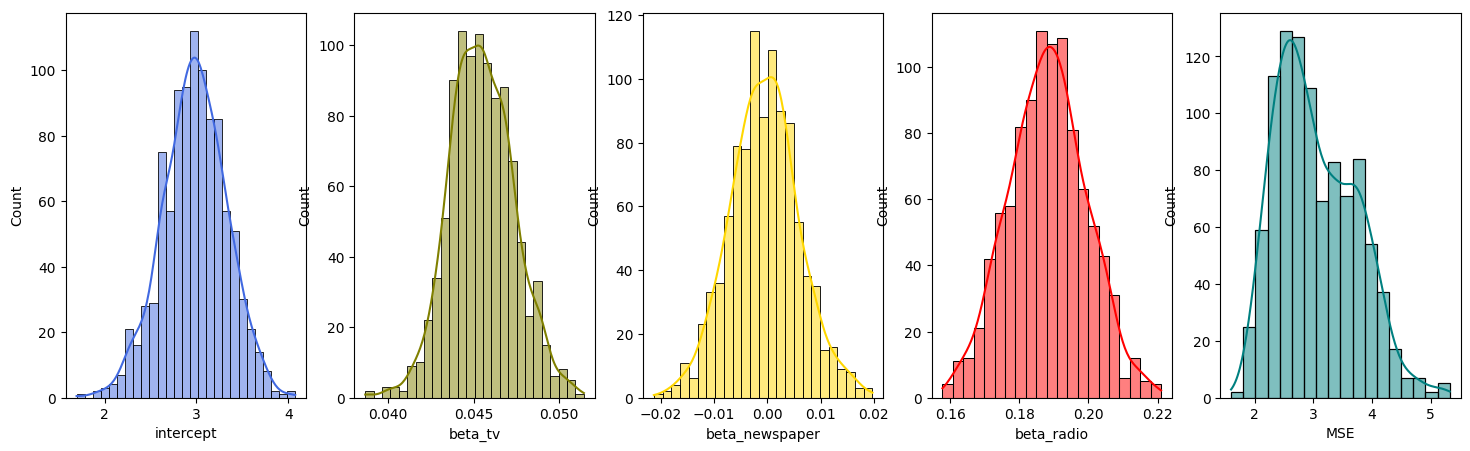
3. Apply bootstrap on the Advertising dataset to fit a multiple linear regressing model using TV, Radio, and newspaper as predictors and sales as a response, and plot the distribution of the bootstrapped estimates of the coefficients and the mean squared error (MSE) test score. Hint: See section 5.2.2

# Write your code below to answer the question

Compare your answer with the reference solution below

import pandas as pd
from sklearn.linear_model import LinearRegression
from sklearn.utils import resample
import matplotlib.pyplot as plt
import seaborn as sns
from sklearn.metrics import mean_squared_error

auto_url = "https://github.com/pykale/transparentML/raw/main/data/Advertising.csv"

ad_df = pd.read_csv(auto_url, na_values="?").dropna()

# Defining number of iterations for bootstrap resample
n_iterations = 1000

# Initializing estimator
lin_reg = LinearRegression()

# Initialising DataFrame, to hold bootstrapped statistics
bootstrapped_stats = pd.DataFrame()

# Each loop iteration is a single bootstrap resample and model fit
for i in range(n_iterations):
    # Sampling n_samples from data, with replacement, as train
    # Defining test to be all observations not in train
    train = resample(ad_df, replace=True, n_samples=len(ad_df))
    test = ad_df[~ad_df.index.isin(train.index)]

    X_train = train.loc[:, ["TV", "Newspaper", "Radio"]]
    y_train = train.loc[:, ["Sales"]]

    X_test = test.loc[:, ["TV", "Newspaper", "Radio"]]
    y_test = test.loc[:, ["Sales"]]

    # Fitting linear regression model
    lin_reg.fit(X_train, y_train)

    # Storing stats in DataFrame, and concatenating with stats
    intercept = lin_reg.intercept_
    beta_tv = lin_reg.coef_.ravel()[0]
    beta_newspaper = lin_reg.coef_.ravel()[1]
    beta_radio = lin_reg.coef_.ravel()[2]

    pred = lin_reg.predict(X_test)
    MSE = mean_squared_error(y_test, pred)

    bootstrapped_stats_i = pd.DataFrame(
        data=dict(
            intercept=intercept,
            beta_tv=beta_tv,
            beta_newspaper=beta_newspaper,
            beta_radio=beta_radio,
            MSE=MSE,
        )
    )

    bootstrapped_stats = pd.concat(objs=[bootstrapped_stats, bootstrapped_stats_i])

# Plotting histograms
fig, axes = plt.subplots(1, 5, figsize=(18, 5))
sns.histplot(bootstrapped_stats["intercept"], color="royalblue", ax=axes[0], kde=True)
sns.histplot(bootstrapped_stats["beta_tv"], color="olive", ax=axes[1], kde=True)
sns.histplot(bootstrapped_stats["beta_newspaper"], color="gold", ax=axes[2], kde=True)
sns.histplot(bootstrapped_stats["beta_radio"], color="red", ax=axes[3], kde=True)
sns.histplot(bootstrapped_stats["MSE"], color="teal", ax=axes[4], kde=True)
plt.show()

previous

5.1. Cross-validation

next

5.3. Quiz and summary