Support vector classifiers
Contents
8.2. Support vector classifiers
This section introduces the concept of an optimal separating hyperplane, the maximal margin classifier, and the support vector classifier, laying the groundwork for the support vector machine. A separating hyperplane is a hyperplane that separates two classes of data. The maximal margin classifier is a separating hyperplane that maximizes the distance between the hyperplane and the nearest data points from either class. The maximal margin classifier is a special case of a support vector machine.
Watch the 11-minute video below for a visual explanation of maximal margin, soft margin, and support vector classifier.
Video
Explaining maximal margin, soft margin, and support vector classifier by StatQuest, embedded according to YouTube’s Terms of Service.
8.2.1. Hyperplane for classification
Firstly, we define a hyperplane and introduce the concept of an optimal separating hyperplane.
8.2.1.1. Hyperplane and its two sides
In a \(D\)-dimensional space, a hyperplane is a flat affine subspace of dimension \(D − 1\). For example, in two dimensions, a hyperplane is a flat one-dimensional subspace—in other words, a line. In three dimensions, a hyperplane is a flat two-dimensional subspace—that is, a plane. In \(D > 3\) dimensions, it can be hard to visualise a hyperplane, but the notion of a \((D − 1)\)-dimensional flat subspace still applies.
The mathematical definition of a hyperplane is quite simple. In two dimensions, a hyperplane is defined by the equation,
where \(\beta_0, \beta_1, \beta_2\) are parameters. When we say that the above equation “defines” the hyperplane, we mean that any \(\mathbf{x} = [x_1, x_2]^\top \) satisfying the equation is a point on the hyperplane. Note the equation above is simply the equation of a line, since indeed in two dimensions a hyperplane is a line. In the \(D\)-dimensional case, the equation defining a hyperplane is
where \(\beta_0, \beta_1, \beta_2, \cdots, \beta_D\) are parameters. In this equation, any \(\mathbf{x} = [x_1, x_2, \cdots, x_D]^\top\) satisfying the above equation is a point on the hyperplane. If \(\mathbf{x} \) does not satisfy the equation, e.g.
then \(\mathbf{x} \) is on one side of the hyperplane, and if
then \(\mathbf{x} \) is on the other side of the hyperplane. So we can think of the hyperplane as dividing \(D\)-dimensional space into two halves. One can easily determine on which side of the hyperplane a point lies by simply calculating the sign of the left hand side of the hyperplane equation.
8.2.1.2. Classification using a separating hyperplane
Suppose we have a set of observations (samples) \(\mathbf{x}_1, \mathbf{x}_2, \cdots, \mathbf{x}_N\) in \(D\)-dimensional space
These observations fall into two classes, \(y_1, \cdots, y_N \in \{-1, 1\}\), where 1 represents one class and -1 the other class. We also have a test observation \( \mathbf{x}^* = [x^*_1, \cdots, x^*_N]^\top\) that we would like to classify. We can do so by finding the hyperplane that separates the two classes. Such a hyperplane is known as a separating hyperplane. Fig. 8.1 below shows a hyperplane in two dimensions.

Fig. 8.1 The hyperplane \(1 + 2x_1 + 3x_2 = 0\) is shown. The blue region (top right) is the set of points for which \(1 + 2x_1 + 3x_2 > 0\), and the purple region (bottom left) is the set of points for which \(1 + 2x_1 + 3x_2\) < 0 (source of figures in this section: https://trevorhastie.github.io/ISLR/).
We can label the observations from the blue class as \( y_n = 1 \) and those from the purple class as \( y_n = −1 \). Then a separating hyperplane has the property that
and
Equivalently, we can write this compactly as

Fig. 8.2 Two classes of observations are shown in blue and in purple, respectively. Left: Three separating hyperplanes, out of many possible, are shown in black. Right: A separating hyperplane is shown in black. The blue and purple grid indicates the decision rule made by a classifier based on this separating hyperplane: a test observation that falls in the blue portion of the grid will be assigned to the blue class, and one that falls in the purple portion of the grid will be assigned to the purple class.
As shown in Fig. 8.2 above, if a separating hyperplane exists, we can use it to construct a very natural classifier: a test observation is assigned a class depending on which side of the hyperplane it is located.
8.2.1.3. The maximal margin classifier (hard margin)
In general, if the data can be perfectly separated using a hyperplane, then there will in fact exist an infinite number of such hyperplanes. This is because a given separating hyperplane can usually be shifted a tiny bit up or down, or rotated, without coming into contact with any of the observations.
A natural choice is the maximal margin hyperplane (also known as the optimal separating hyperplane), which is the separating hyperplane that is farthest from the training observations. That is, we can compute the (perpendicular) distance from each training observation to a given separating hyperplane; the smallest such distance is the minimal distance from the observations to the hyperplane, and is known as the margin. The maximal margin hyperplane is the separating hyperplane for which the margin is largest, i.e. the hyperplane that has the farthest minimum distance to the training observations. We can then classify a test observation based on which side of the maximal margin hyperplane it lies. This is known as the maximal margin classifier. We hope that a classifier that has a large margin on the training data will also have a large margin on the test data, and hence will classify the test observations correctly.

Fig. 8.3 Two classes of observations are shown in blue and in purple, respectively. The maximal margin hyperplane is shown as a solid line. The margin is the distance from the solid line to either of the dashed lines. The two blue points and the purple point that lie on the dashed lines are the support vectors, and the distance from those points to the hyperplane is indicated by arrows. The purple and blue grid indicates the decision rule made by a classifier based on this separating hyperplane.
Fig. 8.3 above shows a maximal margin hyperplane. Comparing to the right-hand panel of Fig. 8.2, we see that the maximal margin hyperplane in Fig. 8.3 results in a greater minimal distance between the observations and the separating hyperplane, i.e. a larger margin. We can also see that three training observations are equidistant from the maximal margin hyperplane and lie along the dashed lines indicating the width of the margin. These three observations are known as support vectors, and the distance from the support vectors to the hyperplane is known as the margin width.
8.2.1.4. Construction of maximal margin classifier
The maximal margin hyperplane is the solution to the following optimisation problem
where \( y_n(\beta_0 + \beta_1 x_{n1} + \beta_2 x_{n2} + \cdots + \beta_D x_{nD}) \) in the constraint represents the perpendicular distance from the \(n\text{th}\) observation to the hyperplane. This constraint guarantees that each observation is on the correct side of the hyperplane and at least a distance \( M \) from the hyperplane. Therefore, \(M\) represents the margin of our hyperplane, and the optimisation problem chooses \( \beta_0, \beta_1, \cdots, \beta_D \) to maximise M. This is exactly the definition of the maximal margin hyperplane! The problem (8.4) can be solved efficiently via quadratic programming, but details of this optimisation are outside of the scope of this course.
8.2.2. Support vector classifier (soft margin)
8.2.2.1. The non-separable case
The maximal margin classifier is a very natural way to perform classification, if a separating hyperplane exists. However, in many cases, no separating hyperplane exists, and so there is no maximal margin classifier. For the example in Fig. 8.4 below, the observations that belong to two classes are not separable by a hyperplane.

Fig. 8.4 Two classes of observations are shown in blue and in purple, respectively. The two classes are not separable by a hyperplane, and so the maximal margin classifier cannot be used.
Even if a separating hyperplane does exist, it is also possible that a classifier based on a separating hyperplane might not be desirable. As shown in the example in Fig. 8.5 below, a classifier based on a separating hyperplane perfectly classifying all of the training observations can lead to sensitivity to individual observations, a symptom of overfitting.
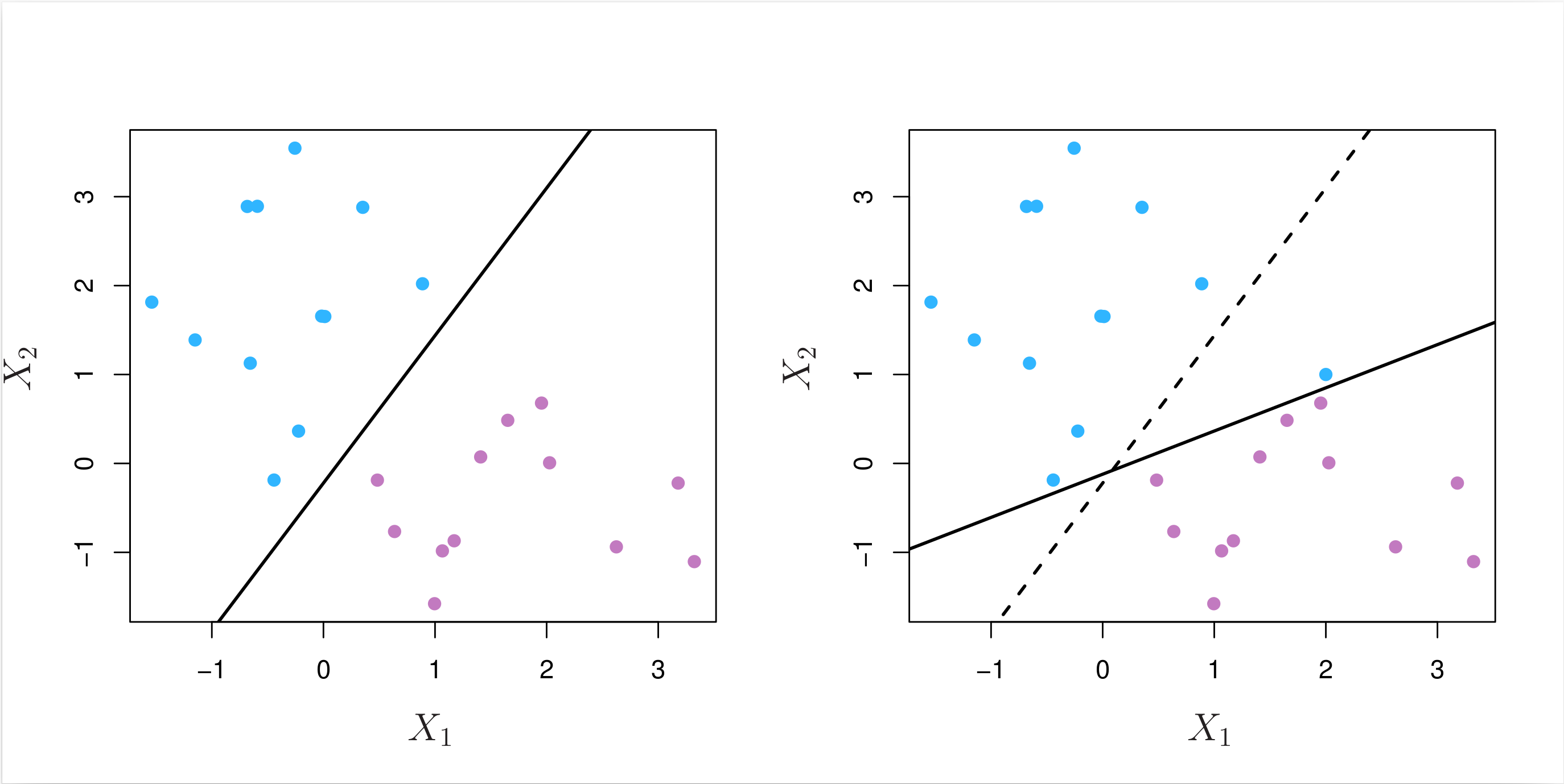
Fig. 8.5 Left: Two classes of observations are shown in blue and in purple, along with the maximal margin hyperplane. Right: An additional blue observation has been added, leading to a dramatic shift in the maximal margin hyperplane shown as a solid line. The dashed line indicates the maximal margin hyperplane that was obtained in the absence of this additional point.
As we can see, the addition of a single observation in the right panel of Fig. 8.5 leads to a dramatic change in the maximal margin hyperplane, and the resulting maximal margin hyperplane has only a tiny margin. As the distance of an observation from the hyperplane can be seen as a measure of our confidence that the observation was correctly classified, this tiny margin indicates that the classifier is not very confident about its classification of the training observations.
Based on the above observations, we might be willing to consider allowing some observations to be on the incorrect side of the margin, or even the incorrect side of the hyperplane, rather than seeking the largest possible margin so that every observation is not only on the correct side of the hyperplane but also on the correct side of the margin. This is the idea behind the support vector classifier, also known as the soft margin classifier.
An example is shown in the left-hand panel of Fig. 8.6 below. Most of the observations are on the correct side of the margin. However, a small subset of the observations (1 and 8) are on the wrong side of the margin.
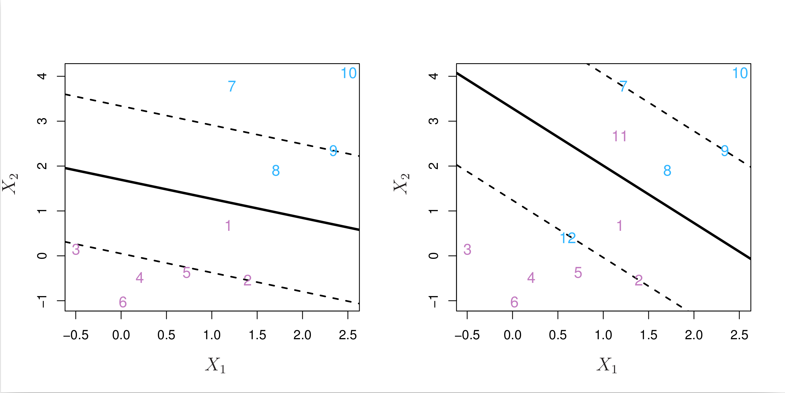
Fig. 8.6 Left: A support vector classifier was fit to a small dataset. The hyperplane is shown as a solid line and the margins are shown as dashed lines. Purple observations: Observations 3, 4, 5, and 6 are on the correct side of the margin, observation 2 is on the margin, and observation 1 is on the wrong side of the margin. Blue observations: Observations 7 and 10 are on the correct side of the margin, observation 9 is on the margin, and observation 8 is on the wrong side of the margin. No observations are on the wrong side of the hyperplane. Right: Same as left panel with two additional points, 11 and 12. These two observations are on the wrong side of the hyperplane and the wrong side of the margin.
An observation can be not only on the wrong side of the margin, but also on the wrong side of the hyperplane. In fact, when there is no separating hyperplane, such a situation is inevitable. Observations on the wrong side of the hyperplane correspond to training observations that are misclassified by the support vector classifier. The right-hand panel of Fig. 8.6 above illustrates such a scenario.
8.2.2.2. Construction of support vector classifier
The support vector classifier classifies a test observation depending on which side of a hyperplane it lies. The hyperplane is chosen to correctly separate most of the training observations into the two classes, but may misclassify a few observations. It is the solution to the “soft margin” optimisation problem below that is a modification of the “hard margin” optimisation problem (8.4) for the maximal margin classifier:
where \( \epsilon_n \) is a slack variable that measures the amount by which the \(n\text{th}\) observation is on the wrong side of the margin. The slack variables are constrained to be non-negative, and the constraint \( \sum_{n = 1}^N \epsilon_n \leq \Omega \) places an upper bound on the total amount by which the observations can be on the wrong side of the margin. The parameter \( \Omega \) is a tuning (hyper)parameter that controls the trade-off between the two competing goals of the support vector classifier: maximising the margin and minimising the number of training observations that are misclassified. \( \Omega \) can also be viewed as a budget for the amount that the margin can be violated by the observations. When \( \Omega \) is very large (highly tolerant), the support vector classifier will attempt to maximise the margin, and so it will misclassify a larger number of training observations. When \( \Omega \) is very small (highly intolerant), the support vector classifier will attempt to minimise the number of training observations that are misclassified, and so it will have a smaller margin. In practice, \( \Omega \) is often tuned using cross-validation. Fig. 8.7 below illustrates the effect of \( \Omega \) on the support vector classifier.
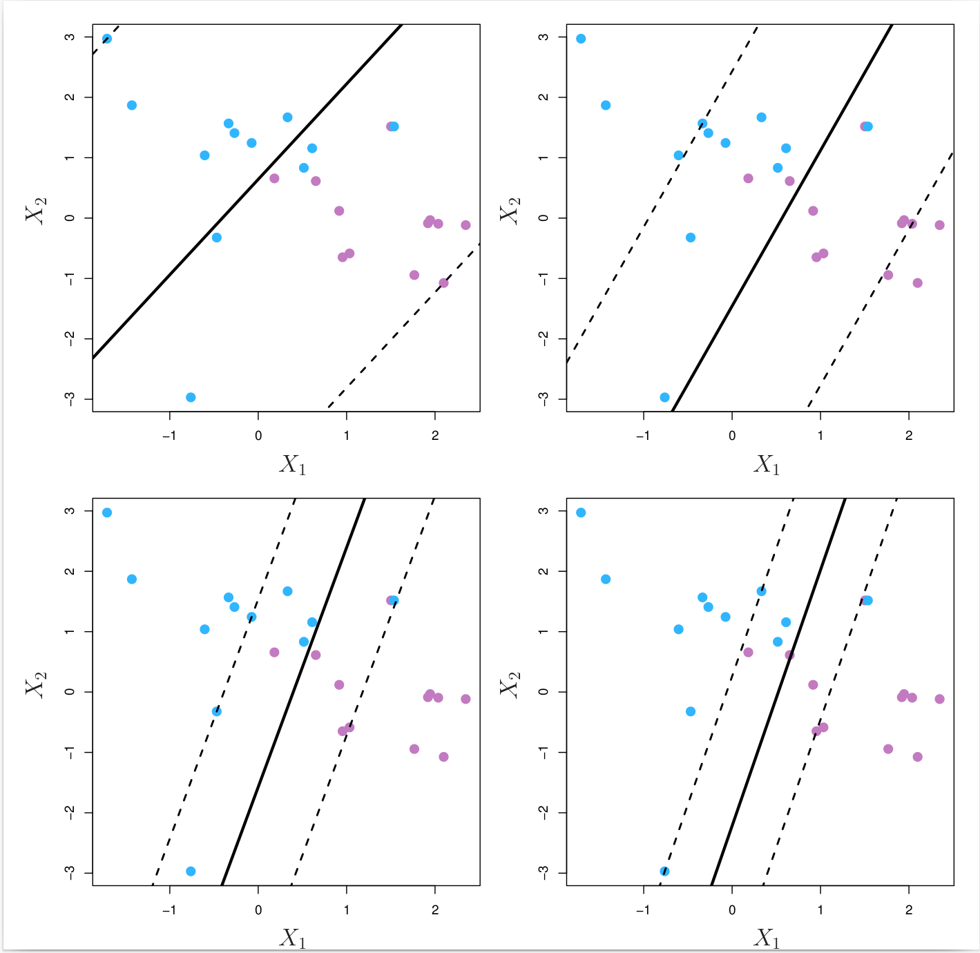
Fig. 8.7 A support vector classifier was fit using four different values of the tuning parameter \( \Omega \) of Equation (8.5). The largest value of \( \Omega \) was used in the top left panel, and smaller values were used in the top right, bottom left, and bottom right panels. When \( \Omega \) is large, then there is a high tolerance for observations being on the wrong side of the margin, and so the margin will be large. As \( \Omega \) decreases, the tolerance for observations being on the wrong side of the margin decreases, and the margin narrows.
8.2.3. Example: support vector classifiers on toy data
In this example, we will use the scikit-learn package to fit support vector classifiers to a small toy dataset.
Get ready by importing the APIs needed from respective libraries.
import pandas as pd
import numpy as np
import matplotlib.pyplot as plt
import seaborn as sns

from sklearn.preprocessing import label_binarize
from sklearn.model_selection import GridSearchCV
from sklearn.svm import SVC, LinearSVC
from sklearn.discriminant_analysis import LinearDiscriminantAnalysis
from sklearn.metrics import (
    confusion_matrix,
    ConfusionMatrixDisplay,
    roc_curve,
    auc,
    classification_report,
)

%matplotlib inline
Define a function to plot a classifier with support vectors.
def plot_svc(svc, X, y, h=0.02, pad=0.25, show=True):
    x_min, x_max = X[:, 0].min() - pad, X[:, 0].max() + pad
    y_min, y_max = X[:, 1].min() - pad, X[:, 1].max() + pad
    xx, yy = np.meshgrid(np.arange(x_min, x_max, h), np.arange(y_min, y_max, h))
    Z = svc.predict(np.c_[xx.ravel(), yy.ravel()])
    Z = Z.reshape(xx.shape)
    plt.contourf(xx, yy, Z, cmap=plt.cm.Paired, alpha=0.2)

    plt.scatter(X[:, 0], X[:, 1], s=70, c=y, cmap=plt.cm.Paired)
    # Support vectors indicated in plot by vertical lines
    sv = svc.support_vectors_
    plt.scatter(
        sv[:, 0], sv[:, 1], c="k", marker="x", s=100, alpha=0.5
    )  # , linewidths=1)
    plt.xlim(x_min, x_max)
    plt.ylim(y_min, y_max)
    plt.xlabel("X1")
    plt.ylabel("X2")
    print("Number of support vectors: ", svc.support_.size)
    if show:
        plt.show()
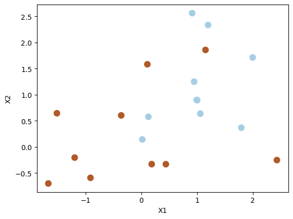
Generate synthetic data randomly: 20 observations of 2 features and divide into two classes. Set a seed for reproducibility.
np.random.seed(5)
X = np.random.randn(20, 2)
y = np.repeat([1, -1], 10)

X[y == -1] = X[y == -1] + 1
plt.scatter(X[:, 0], X[:, 1], s=70, c=y, cmap=plt.cm.Paired)
plt.xlabel("X1")
plt.ylabel("X2")
plt.show()
y
array([ 1,  1,  1,  1,  1,  1,  1,  1,  1,  1, -1, -1, -1, -1, -1, -1, -1,
       -1, -1, -1])
8.2.3.1. Support vector visualisation and interpretation
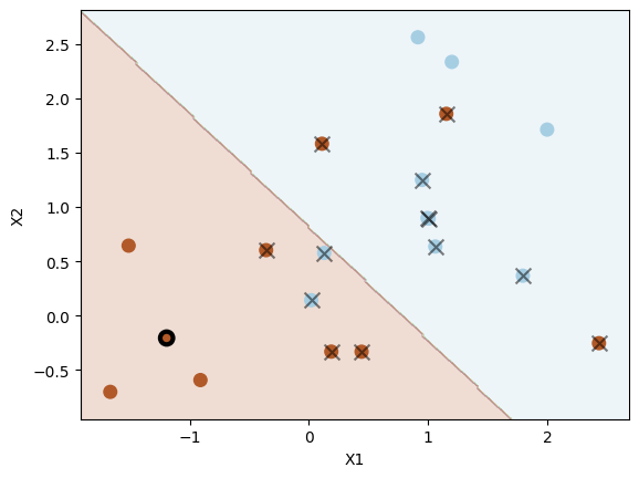
Fit a support vector classifier and visualise decision boundary and support vectors with data points. We will study different values of hyperparameter \( \Omega \) in Equation (8.5) to see its effect on the decision boundary.
Note: The C setting of the SVC class in scikit-learn is inversely proportional to \( \Omega \). The larger the value of C, the smaller the value of \( \Omega \) (the less tolerance for observations being on the wrong side of the margin). The smaller the value of C, the larger the value of \( \Omega \) (the more tolerance for observations being on the wrong side of the margin).
svc = SVC(C=1.0, kernel="linear")
svc.fit(X, y)

plot_svc(svc, X, y, show=False)
plt.scatter(
    X[5, 0], X[5, 1], s=70, facecolors="none", marker="o", edgecolors="k", linewidths=3
)
plt.show()
Number of support vectors: 13
print("Input: ", X[5, :])
print("Intercept: ", svc.intercept_[0], " Coefficients: ", svc.coef_[0])
print("Prediction score: ", svc.decision_function(X[5, :].reshape(1, -1))[0])
print("Prediction: ", svc.predict(X[5, :].reshape(1, -1))[0])
Input:  [-1.19276461 -0.20487651]
Intercept:  0.5729441305210916  Coefficients:  [-0.73273926 -0.70326681]
Prediction score:  1.5910124372951457
Prediction:  1
System transparency
The coefficients of the support vector classifier are \( \beta_0 \approx 0.5729, \beta_1 \approx -0.7327, \beta_2 \approx -0.7033 \)
For the data point \([-1.19276461, -0.20487651]\) marked by a black circle, its prediction score is \( -0.7327 \times -1.19276461 + -0.7033 \times -0.20487651 + 0.5729 \approx 1.5910 \), which is positive. So the predicted label is \( 1 \).
According to the definition, the data points on the hyperplane satisfies \( \beta_0 + \beta_1 x_{1} + \beta_2 x_{2} = 0 \), i.e. \( 0.5729 -0.7327 \times x_1 -0.7033 \times x_2 = 0 \). To get a data point \( \mathbf{x} = [x_1, x_2]^\top \) of class \( 1 \), the relationship between \( x_1 \) and \( x_2 \) should satisfy:
Similarly, we need data points \( \mathbf{x} = [x_1, x_2]^\top \) satisfy \( x_1 < 0.7819 - 0.9598 \times x_2 \) for class \( -1 \). Note that the data point \( \mathbf{x} = [x_1, x_2]^\top \) belongs to class \( 1 \) but violates the margin if \( 0 < 0.5729 -0.7327 \times x_1 -0.7033 \times x_2 < 1 \), and the same applies to data points belongs to class \( -1 \) if \( -1 < 0.5729 -0.7327 \times x_1 -0.7033 \times x_2 < 0 \).
Let us use a smaller value of \( \Omega \) (C=0.1) to see how the decision boundary changes.
svc2 = SVC(C=0.1, kernel="linear")
svc2.fit(X, y)
plot_svc(svc2, X, y)
Number of support vectors: 16

As shown above, when using a smaller C=0.1, we have a larger \( \Omega \) and a larger tolerance for observations being on the wrong side of the margin. As a result, the margin is wider, resulting in more support vectors. We can select the optimal hyperparameter C in scikit-learn (inversely proportional to \( \Omega \)) using cross-validation, as we do below using GridSearchCV from scikit-learn.
tuned_parameters = [{"C": [0.001, 0.01, 0.1, 1, 5, 10, 100]}]
clf = GridSearchCV(
    SVC(kernel="linear"),
    tuned_parameters,
    cv=10,
    scoring="accuracy",
    return_train_score=True,
)
clf.fit(X, y)
clf.cv_results_
{'mean_fit_time': array([0.00063426, 0.00059206, 0.00057888, 0.00060322, 0.00060067,
        0.0005976 , 0.0007026 ]),
 'std_fit_time': array([1.01430395e-04, 2.82656362e-05, 1.01365756e-05, 5.24885365e-05,
        1.66504954e-05, 6.84410837e-06, 3.75261225e-05]),
 'mean_score_time': array([0.00055819, 0.00051837, 0.00051835, 0.00052588, 0.00051618,
        0.00052531, 0.00051625]),
 'std_score_time': array([1.02414742e-04, 1.03473663e-05, 9.96717988e-06, 1.07389244e-05,
        3.98808082e-06, 1.80683063e-05, 3.62215813e-06]),
 'param_C': masked_array(data=[0.001, 0.01, 0.1, 1, 5, 10, 100],
              mask=[False, False, False, False, False, False, False],
        fill_value='?',
             dtype=object),
 'params': [{'C': 0.001},
  {'C': 0.01},
  {'C': 0.1},
  {'C': 1},
  {'C': 5},
  {'C': 10},
  {'C': 100}],
 'split0_test_score': array([0.5, 0.5, 0.5, 0.5, 0.5, 0.5, 0.5]),
 'split1_test_score': array([0.5, 0.5, 0.5, 0. , 0. , 0. , 0. ]),
 'split2_test_score': array([0.5, 0.5, 0.5, 0.5, 0.5, 0.5, 0.5]),
 'split3_test_score': array([1., 1., 1., 1., 1., 1., 1.]),
 'split4_test_score': array([1., 1., 1., 1., 1., 1., 1.]),
 'split5_test_score': array([1., 1., 1., 1., 1., 1., 1.]),
 'split6_test_score': array([1., 1., 1., 1., 1., 1., 1.]),
 'split7_test_score': array([1., 1., 1., 1., 1., 1., 1.]),
 'split8_test_score': array([0.5, 0.5, 0.5, 0.5, 0.5, 0.5, 0.5]),
 'split9_test_score': array([1., 1., 1., 1., 1., 1., 1.]),
 'mean_test_score': array([0.8 , 0.8 , 0.8 , 0.75, 0.75, 0.75, 0.75]),
 'std_test_score': array([0.24494897, 0.24494897, 0.24494897, 0.3354102 , 0.3354102 ,
        0.3354102 , 0.3354102 ]),
 'rank_test_score': array([1, 1, 1, 4, 4, 4, 4], dtype=int32),
 'split0_train_score': array([0.83333333, 0.83333333, 0.77777778, 0.77777778, 0.77777778,
        0.77777778, 0.77777778]),
 'split1_train_score': array([0.83333333, 0.83333333, 0.83333333, 0.88888889, 0.88888889,
        0.88888889, 0.88888889]),
 'split2_train_score': array([0.83333333, 0.83333333, 0.77777778, 0.83333333, 0.83333333,
        0.83333333, 0.83333333]),
 'split3_train_score': array([0.77777778, 0.77777778, 0.72222222, 0.72222222, 0.72222222,
        0.72222222, 0.72222222]),
 'split4_train_score': array([0.77777778, 0.77777778, 0.72222222, 0.77777778, 0.77777778,
        0.77777778, 0.77777778]),
 'split5_train_score': array([0.77777778, 0.77777778, 0.72222222, 0.72222222, 0.72222222,
        0.72222222, 0.72222222]),
 'split6_train_score': array([0.77777778, 0.77777778, 0.72222222, 0.77777778, 0.72222222,
        0.72222222, 0.72222222]),
 'split7_train_score': array([0.72222222, 0.72222222, 0.72222222, 0.77777778, 0.72222222,
        0.72222222, 0.72222222]),
 'split8_train_score': array([0.83333333, 0.83333333, 0.77777778, 0.77777778, 0.77777778,
        0.77777778, 0.77777778]),
 'split9_train_score': array([0.77777778, 0.77777778, 0.72222222, 0.72222222, 0.72222222,
        0.72222222, 0.72222222]),
 'mean_train_score': array([0.79444444, 0.79444444, 0.75      , 0.77777778, 0.76666667,
        0.76666667, 0.76666667]),
 'std_train_score': array([0.03557291, 0.03557291, 0.0372678 , 0.0496904 , 0.05443311,
        0.05443311, 0.05443311])}
Display the optimal hyperparameter C in scikit-learn (inversely proportional to \( \Omega \)).
clf.best_params_
{'C': 0.001}
8.2.3.2. Prediction with support vector classifiers
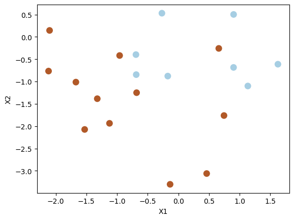
Generate a test dataset.
np.random.seed(1)
X_test = np.random.randn(20, 2)
y_test = np.random.choice([-1, 1], 20)
X_test[y_test == 1] = X_test[y_test == 1] - 1

plt.scatter(X_test[:, 0], X_test[:, 1], s=70, c=y_test, cmap=plt.cm.Paired)
plt.xlabel("X1")
plt.ylabel("X2")
plt.show()
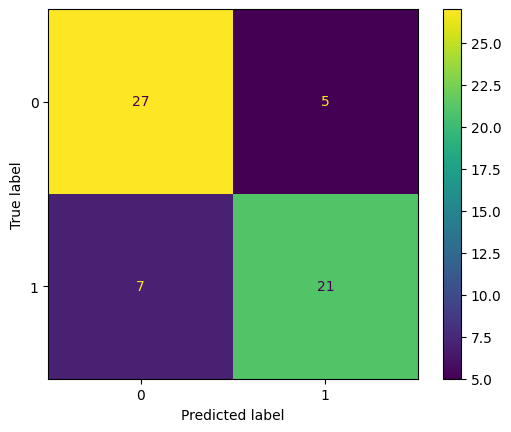
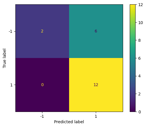
Predict the class labels for the test dataset and display the confusion matrix.
# svc2 : C = 0.1
y_pred = svc2.predict(X_test)
cm = confusion_matrix(y_test, y_pred)
disp = ConfusionMatrixDisplay(confusion_matrix=cm, display_labels=svc.classes_)
disp.plot()
plt.show()
Repeat with a smaller value of C (larger \( \Omega \) and larger tolerance) to see how the confusion matrix changes.
svc3 = SVC(C=0.001, kernel="linear")
svc3.fit(X, y)

y_pred = svc3.predict(X_test)
cm = confusion_matrix(y_test, y_pred)
disp = ConfusionMatrixDisplay(confusion_matrix=cm, display_labels=svc.classes_)
disp.plot()
plt.show()

The prediction results are the same as the previous case for this particular example.
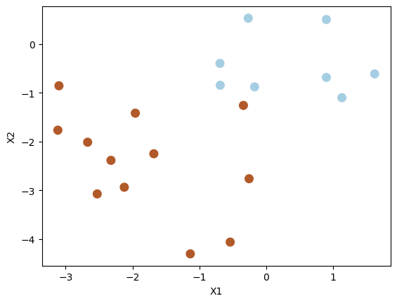
8.2.3.3. Decision boundary on linearly separable data
Let us modify the test dataset so that the classes are linearly separable with a hyperplane.
X_test[y_test == 1] = X_test[y_test == 1] - 1
plt.scatter(X_test[:, 0], X_test[:, 1], s=70, c=y_test, cmap=plt.cm.Paired)
plt.xlabel("X1")
plt.ylabel("X2")
plt.show()
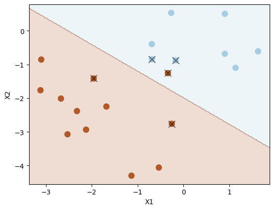
Set C to be very large (meaning small \( \Omega \) and small tolerance) to see whether the decision boundary can separate the two classes perfectly.
svc4 = SVC(C=10.0, kernel="linear")
svc4.fit(X_test, y_test)
plot_svc(svc4, X_test, y_test)
Number of support vectors: 4
Indeed, we have a perfect separation of the two classes.
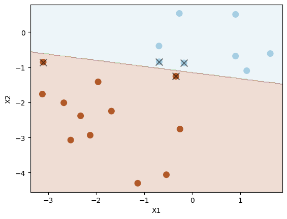
Let us increase the margin tolerance (reduce C in scikit-learn) to see how the decision boundary changes.
svc5 = SVC(C=1, kernel="linear")
svc5.fit(X_test, y_test)
plot_svc(svc5, X_test, y_test)
Number of support vectors: 5
Now there is one misclassification. Thus, this version (with C=1) has lowered variance (and overfitting) at the expense of increased bias.
8.2.4. Exercises
1. All the following exercises use the Heart dataset.
Load the Heart dataset, convert the values of variables (predictors) from categorical values to numerical values, and inspect the first five rows.
# Write your code below to answer the question
Compare your answer with the reference solution below
import numpy as np
import pandas as pd

np.random.seed(2022)

heart_url = "https://github.com/pykale/transparentML/raw/main/data/Heart.csv"

heart_df = pd.read_csv(heart_url, index_col=0).dropna()
# converting categories
heart_df["ChestPain"] = heart_df["ChestPain"].factorize()[0]
heart_df["Thal"] = heart_df["Thal"].factorize()[0]
heart_df["AHD"] = heart_df["AHD"].factorize()[0]

heart_df.head(5)
| Age | Sex | ChestPain | RestBP | Chol | Fbs | RestECG | MaxHR | ExAng | Oldpeak | Slope | Ca | Thal | AHD | |
|---|---|---|---|---|---|---|---|---|---|---|---|---|---|---|
| 1 | 63 | 1 | 0 | 145 | 233 | 1 | 2 | 150 | 0 | 2.3 | 3 | 0.0 | 0 | 0 |
| 2 | 67 | 1 | 1 | 160 | 286 | 0 | 2 | 108 | 1 | 1.5 | 2 | 3.0 | 1 | 1 |
| 3 | 67 | 1 | 1 | 120 | 229 | 0 | 2 | 129 | 1 | 2.6 | 2 | 2.0 | 2 | 1 |
| 4 | 37 | 1 | 2 | 130 | 250 | 0 | 0 | 187 | 0 | 3.5 | 3 | 0.0 | 1 | 0 |
| 5 | 41 | 0 | 3 | 130 | 204 | 0 | 2 | 172 | 0 | 1.4 | 1 | 0.0 | 1 | 0 |
2. Split the loaded dataset into training and testing sets in an \(80:20\) ratio, then train a model using SVC using the hyperparameter \(C = 1\), and show the number of support vectors and accuracy of this trained model on the test set. (Use \(2022\) as the random seed value)
# Write your code below to answer the question
Compare your answer with the reference solution below
from sklearn.svm import SVC
from sklearn.model_selection import train_test_split
from sklearn.metrics import accuracy_score

np.random.seed(2022)

X = heart_df.drop(["AHD"], axis=1)
y = heart_df["AHD"]


X_train, X_test, y_train, y_test = train_test_split(
    X, y.ravel(), test_size=0.2, random_state=2022
)

svc = SVC(C=1, kernel="linear", random_state=2022)
svc.fit(X_train, y_train)

print("Number of Support vectors: ", len(svc.support_vectors_))

y_pred = svc.predict(X_test)
accuracy = accuracy_score(y_test, y_pred)

print("Accuracy: ", accuracy)
Number of Support vectors:  96
Accuracy:  0.7666666666666667
3. Train another model in the same manner as in Exercise 2, but with the hyperparameter regularisation strength \(C\) set to \(0.01\). Show the number of support vectors and accuracy of this trained model on the test set.
# Write your code below to answer the question
Compare your answer with the reference solution below
svc2 = SVC(C=0.01, kernel="linear", random_state=2022)
svc2.fit(X_train, y_train)
print("Number of Support vectors: ", len(svc2.support_vectors_))

y_pred = svc2.predict(X_test)
accuracy = accuracy_score(y_test, y_pred)

print("Accuracy: ", accuracy)
Number of Support vectors:  149
Accuracy:  0.7833333333333333
4. Using GridSearchCV, fine-tune the support vector classifier’s hyperparameter \(C\) on the training dataset (using \(10\)-fold cross-validation) for \(C\) values of \(0.001\), \(0.01\), \(0.1\), and \(5\), and then display the best hyperparameters. (Use the accuracy scoring for choosing the best model and its hyperparameters.)
# Write your code below to answer the question
Compare your answer with the reference solution below
from sklearn.model_selection import GridSearchCV

tuned_parameters = [{"C": [0.001, 0.01, 0.1, 1, 5]}]
clf = GridSearchCV(
    SVC(kernel="linear"),
    tuned_parameters,
    cv=10,
    scoring="accuracy",
    return_train_score=True,
)
clf.fit(X, y)
print("\nOptimal value of C : ", clf.best_params_)
Optimal value of C : {'C': 0.1}
5. Finally, using the best hyperparameter from Exercise 4, train another SVC model on the training dataset and show the accuracy of this trained model on the test set. Also, show the confusion matrix for this trained model.
# Write your code below to answer the question
Compare your answer with the reference solution below
import matplotlib.pyplot as plt
from sklearn.metrics import confusion_matrix, ConfusionMatrixDisplay, roc_curve, auc

svc_tuned = SVC(C=0.1, kernel="linear")
svc_tuned.fit(X_train, y_train)
print("Number of Support vectors: ", len(svc_tuned.support_vectors_))

y_pred = svc_tuned.predict(X_test)
accuracy = accuracy_score(y_test, y_pred)

print("Accuracy: ", accuracy)

cm = confusion_matrix(y_test, y_pred)
disp = ConfusionMatrixDisplay(confusion_matrix=cm, display_labels=svc_tuned.classes_)
disp.plot()
plt.show()
Number of Support vectors:  111
Accuracy:  0.8