Support vector machines
Contents
8.3. Support vector machines
This section introduces support vector machines (SVMs) for nonlinear classification.
Watch the 9-minute video below for a visual explanation of nonlinear (polynomial) kernel and SVM.
Video
Explaining nonlinear (polynomial) kernel and SVM by StatQuest, embedded according to YouTube’s Terms of Service.
8.3.1. Classification with nonlinear decision boundaries
In binary classification, if the boundary between the two classes is linear, the support vector classifier is a natural approach. However, in practice, two classes may have nonlinear boundaries between them, as the example shown in the left panel of Fig. 8.8 below.
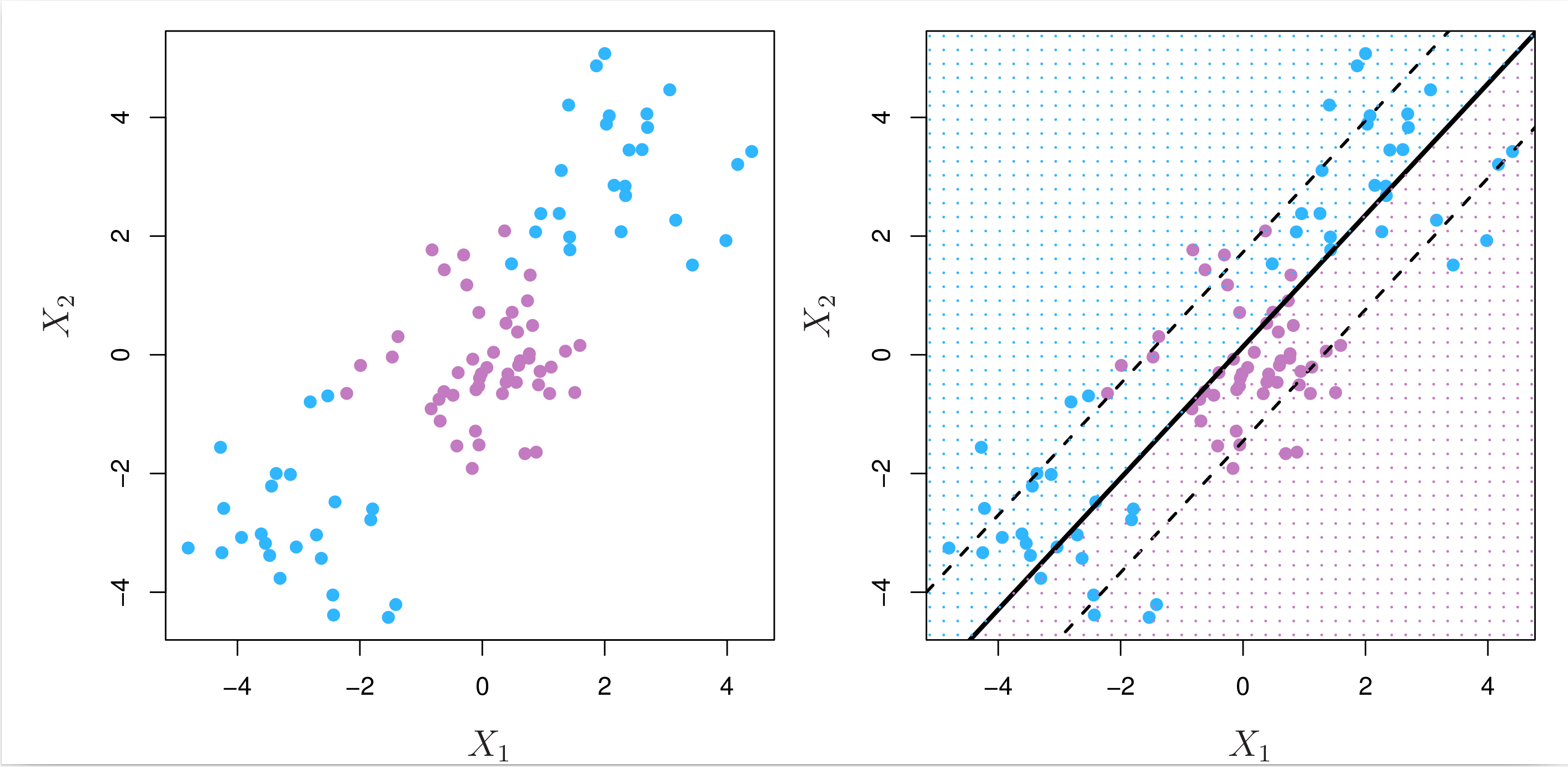
Fig. 8.8 Left: The observations fall into two classes, with a nonlinear boundary between them. Right: The support vector classifier seeks a linear boundary, and consequently performs very poorly.
In Linear regression, we discussed using higher-order polynomials as a way to fit a nonlinear relationship between the input features (predictors) and the output (response). Likewise, rather than fitting a support vector classifier using \(D\) features: \( x_{1}, x_{2}, \cdots, x_{D} \), we could fit a support vector classifier using \( 2 \times D \) features: \( x_{1}, x_{2}, \cdots, x_{D'}, x_{1}^2, x_{2}^2, \cdots, x_{D'}^2 \). Then the optimisation problem becomes
The decision boundary that results from Equation (8.7) is in fact linear in the enlarged (augmented) features space of 2D features. But in the original feature space of \(D\) features, the decision boundary is of the form \( q(\mathbf{x}) = 0 \), where \( q(\cdot) \) is a quadratic polynomial, so its solutions are generally nonlinear.
8.3.2. Kernel methods
The support vector machine (SVM) extends the support vector classifier by enlarging the feature space in a specific way, using kernels. As in the above example of using quadratic terms, the main idea is to enlarge the feature space in order to accommodate a nonlinear boundary between the classes. The kernel approach is simply a computationally efficient approach for this idea.
Exactly how the support vector classifier is computed is too technical to cover here. One fact from the solution to support vector classifier problem (8.5) is that it involves only the inner products of the input features (observations), as opposed to the features themselves.
The inner product of two \(D\)-vectors \(\mathbf{a}\) and \(\mathbf{b}\) is defined as \(⟨\mathbf{a}, \mathbf{b}⟩ = \sum_{d = 1}^{D} a_d b_d \). Thus, the inner product of two observations \(\mathbf{x}_n\) and \(\mathbf{x}_{n'}\) is \(⟨\mathbf{x}_n, \mathbf{x}_{n'}⟩ = \sum_{d = 1}^{D} x_{nd} x_{n'd} \). As a result, the linear support vector classifier can be written as
where there are \(N\) parameters \(\alpha_n, \text{ for } n = 1, \cdots N \), one per training observation (sample). To estimate the parameters \(\{\alpha_n\}\), all we need are the inner products of the training observations. The inner product can be denoted in the following generalised form:
where \( k(\cdot, \cdot) \) is a kernel function that quantifies the similarity between two observations. For instance, we could simply take
which is the linear kernel for the support vector classifier.
More flexibly, we could also take
which is known as a polynomial kernel of degree \( \tilde{d} \) (a positive integer). Another popular choice is the radial basis function (RBF) kernel or simply radial kernel, which takes the form
where \( \gamma > 0 \) is a positive tuning parameter, i.e. hyperparameter. The radial kernel is also known as the Gaussian kernel. Fig. 8.9 below shows the decision boundaries obtained from using the polynomial (left) and radial kernels (right).
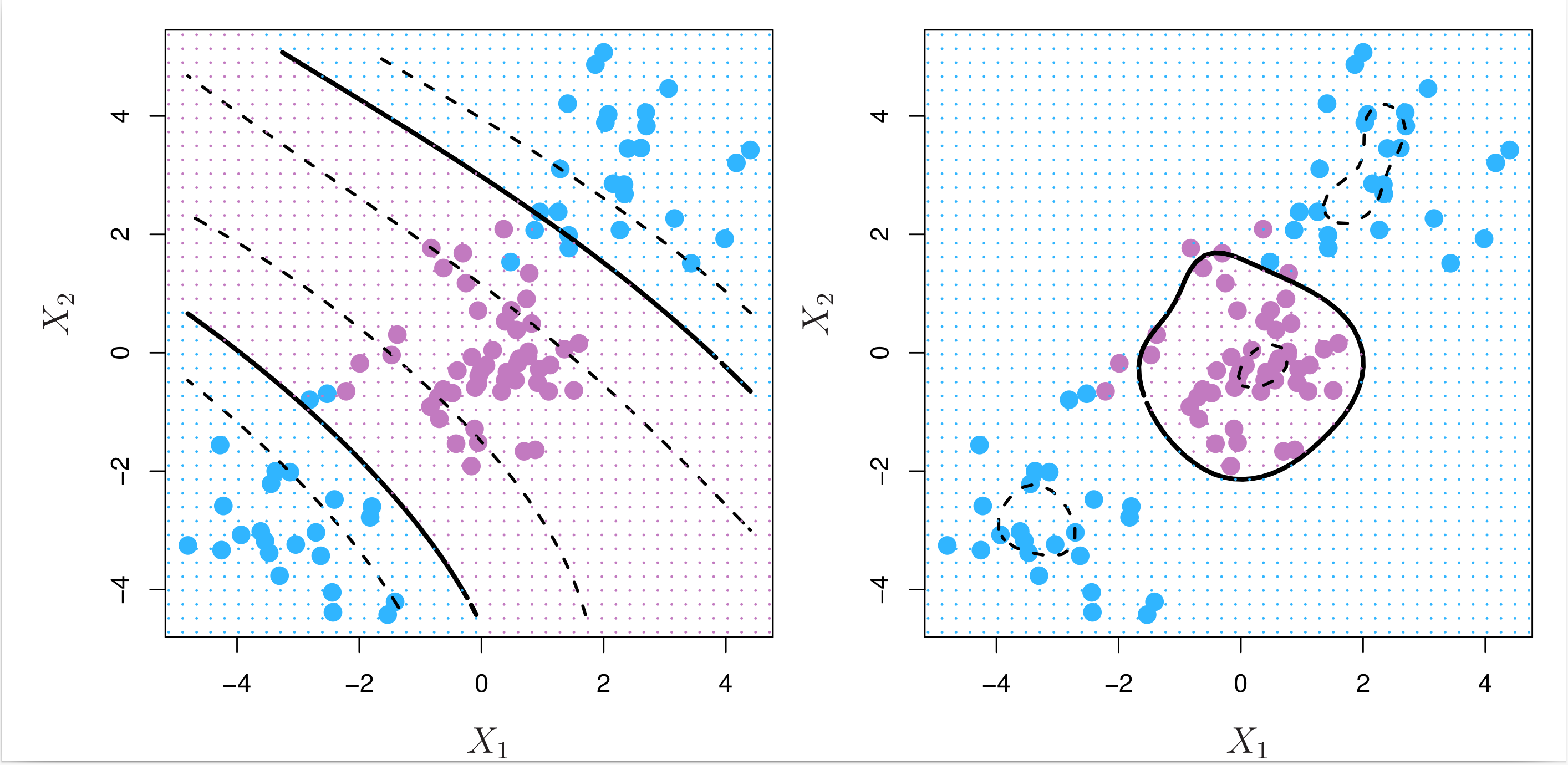
Fig. 8.9 Left: An SVM with a polynomial kernel of degree 3 is applied to the nonlinear data from Fig. 8.8, resulting in a far more appropriate decision rule. Right: An SVM with a radial kernel is applied. In this example, either kernel is capable of capturing the decision boundary.
When the support vector classifier is combined with a nonlinear kernel, the resulting classifier is known as a support vector machine:
8.3.3. Example: support vector machines on toy data
Get ready by importing the APIs needed from respective libraries.
import numpy as np
import matplotlib.pyplot as plt

from sklearn.metrics import confusion_matrix, ConfusionMatrixDisplay, roc_curve, auc
from sklearn.model_selection import train_test_split, GridSearchCV
from sklearn.svm import SVC

%matplotlib inline
Define a function to plot a classifier with support vectors as in the previous section.
def plot_svc(svc, X, y, h=0.02, pad=0.25):
    x_min, x_max = X[:, 0].min() - pad, X[:, 0].max() + pad
    y_min, y_max = X[:, 1].min() - pad, X[:, 1].max() + pad
    xx, yy = np.meshgrid(np.arange(x_min, x_max, h), np.arange(y_min, y_max, h))
    Z = svc.predict(np.c_[xx.ravel(), yy.ravel()])
    Z = Z.reshape(xx.shape)
    plt.contourf(xx, yy, Z, cmap=plt.cm.Paired, alpha=0.2)

    plt.scatter(X[:, 0], X[:, 1], s=70, c=y, cmap=plt.cm.Paired)
    # Support vectors indicated in plot by vertical lines
    sv = svc.support_vectors_
    plt.scatter(
        sv[:, 0], sv[:, 1], c="k", marker="x", s=100, alpha=0.5
    )  # , linewidths=1)
    plt.xlim(x_min, x_max)
    plt.ylim(y_min, y_max)
    plt.xlabel("X1")
    plt.ylabel("X2")
    plt.show()
    print("Number of support vectors: ", svc.support_.size)
8.3.3.1. Training SVMs
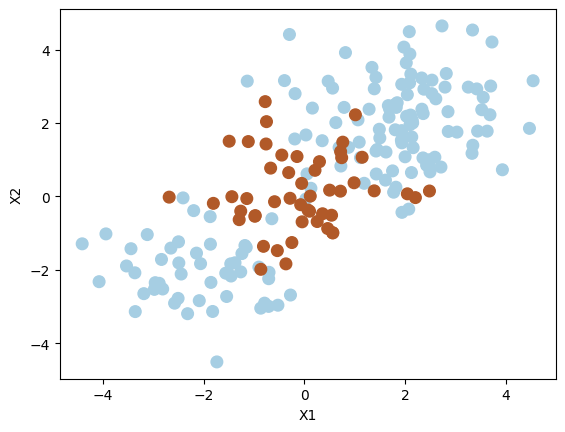
Generate synthetic data randomly. Set a seed for reproducibility.
np.random.seed(8)
X = np.random.randn(200, 2)
X[:100] = X[:100] + 2
X[101:150] = X[101:150] - 2
y = np.concatenate([np.repeat(-1, 150), np.repeat(1, 50)])

X_train, X_test, y_train, y_test = train_test_split(X, y, test_size=0.5, random_state=2)

plt.scatter(X[:, 0], X[:, 1], s=70, c=y, cmap=plt.cm.Paired)
plt.xlabel("X1")
plt.ylabel("X2")
plt.show()
Use the SVC class from sklearn.svm to train a support vector machine with a radial kernel. The C parameter is the inverse of the regularisation strength \( \Omega \), and the gamma parameter is the inverse of the kernel width. The fit method trains the model.
svm = SVC(C=1.0, kernel="rbf", gamma=1)
svm.fit(X_train, y_train)
plot_svc(svm, X_train, y_train)
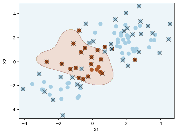
Number of support vectors: 51
Let us reduce the regularisation strength \( \Omega \) by increasing the value of C. This results in a more flexible decision boundary, and will likely overfit the data.
svm2 = SVC(C=100, kernel="rbf", gamma=1)
svm2.fit(X_train, y_train)
plot_svc(svm2, X_train, y_train)
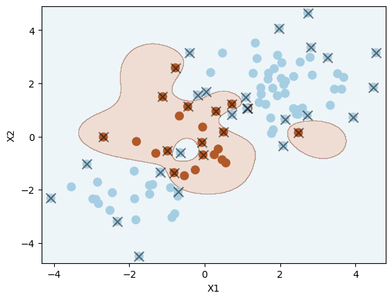
Number of support vectors: 36
Challenge
Can you identify signs of overfitting in the plot?
Choose (tune) the (hyper)parameters C and gamma using cross-validation. The GridSearchCV class from sklearn.model_selection performs a grid search over the specified parameter values. The cv parameter specifies the number of folds in the cross-validation. The fit method trains the model.
tuned_parameters = {"C": [0.01, 0.1, 1, 10, 100], "gamma": [0.5, 1, 2, 3, 4]}
clf = GridSearchCV(
    SVC(kernel="rbf"),
    tuned_parameters,
    cv=10,
    scoring="accuracy",
    return_train_score=True,
)
clf.fit(X_train, y_train)
clf.cv_results_
{'mean_fit_time': array([0.00070751, 0.00068641, 0.00070105, 0.00071216, 0.00072191,
        0.00066285, 0.00069885, 0.00073698, 0.00075343, 0.00076895,
        0.00065999, 0.00069444, 0.00077188, 0.00078981, 0.00080082,
        0.00066903, 0.00071349, 0.00079968, 0.00082698, 0.00082088,
        0.00071986, 0.00074396, 0.00079794, 0.00082898, 0.00081098]),
 'std_fit_time': array([1.01051641e-04, 2.61342001e-05, 1.26322254e-05, 1.35177237e-05,
        1.16447159e-05, 7.13728227e-06, 1.34637064e-05, 3.23757068e-05,
        2.62577667e-05, 6.73995450e-06, 2.05222315e-05, 1.15504144e-05,
        2.35813331e-05, 1.21369108e-05, 1.50144846e-05, 2.53066357e-05,
        2.27886759e-05, 2.73289370e-05, 2.78191065e-05, 1.74110871e-05,
        2.43826684e-05, 3.04730657e-05, 1.41009221e-05, 2.62344954e-05,
        2.05287258e-05]),
 'mean_score_time': array([0.00054493, 0.00054419, 0.00053911, 0.0005414 , 0.00054095,
        0.00053587, 0.0005374 , 0.00053475, 0.00054109, 0.00054238,
        0.00053089, 0.00052695, 0.00053694, 0.00053732, 0.00054586,
        0.0005275 , 0.00053051, 0.00053344, 0.00054264, 0.00053697,
        0.00051775, 0.00051844, 0.00053048, 0.00053582, 0.00054004]),
 'std_score_time': array([2.81627147e-05, 1.23547072e-05, 7.11654498e-06, 8.45078681e-06,
        8.14990592e-06, 1.49293442e-05, 1.02092161e-05, 6.67695477e-06,
        1.32025566e-05, 6.78840123e-06, 1.28640246e-05, 6.04173567e-06,
        1.48511811e-05, 9.43610617e-06, 1.82015839e-05, 1.77179657e-05,
        2.34784686e-05, 1.52353763e-05, 1.72717765e-05, 9.49361107e-06,
        6.91759089e-06, 5.84903510e-06, 1.10776158e-05, 9.68355190e-06,
        1.35921384e-05]),
 'param_C': masked_array(data=[0.01, 0.01, 0.01, 0.01, 0.01, 0.1, 0.1, 0.1, 0.1, 0.1,
                    1, 1, 1, 1, 1, 10, 10, 10, 10, 10, 100, 100, 100, 100,
                    100],
              mask=[False, False, False, False, False, False, False, False,
                    False, False, False, False, False, False, False, False,
                    False, False, False, False, False, False, False, False,
                    False],
        fill_value='?',
             dtype=object),
 'param_gamma': masked_array(data=[0.5, 1, 2, 3, 4, 0.5, 1, 2, 3, 4, 0.5, 1, 2, 3, 4, 0.5,
                    1, 2, 3, 4, 0.5, 1, 2, 3, 4],
              mask=[False, False, False, False, False, False, False, False,
                    False, False, False, False, False, False, False, False,
                    False, False, False, False, False, False, False, False,
                    False],
        fill_value='?',
             dtype=object),
 'params': [{'C': 0.01, 'gamma': 0.5},
  {'C': 0.01, 'gamma': 1},
  {'C': 0.01, 'gamma': 2},
  {'C': 0.01, 'gamma': 3},
  {'C': 0.01, 'gamma': 4},
  {'C': 0.1, 'gamma': 0.5},
  {'C': 0.1, 'gamma': 1},
  {'C': 0.1, 'gamma': 2},
  {'C': 0.1, 'gamma': 3},
  {'C': 0.1, 'gamma': 4},
  {'C': 1, 'gamma': 0.5},
  {'C': 1, 'gamma': 1},
  {'C': 1, 'gamma': 2},
  {'C': 1, 'gamma': 3},
  {'C': 1, 'gamma': 4},
  {'C': 10, 'gamma': 0.5},
  {'C': 10, 'gamma': 1},
  {'C': 10, 'gamma': 2},
  {'C': 10, 'gamma': 3},
  {'C': 10, 'gamma': 4},
  {'C': 100, 'gamma': 0.5},
  {'C': 100, 'gamma': 1},
  {'C': 100, 'gamma': 2},
  {'C': 100, 'gamma': 3},
  {'C': 100, 'gamma': 4}],
 'split0_test_score': array([0.8, 0.8, 0.8, 0.8, 0.8, 0.8, 0.8, 0.8, 0.8, 0.8, 0.9, 0.9, 0.7,
        0.7, 0.7, 0.8, 0.8, 0.7, 0.7, 0.7, 0.8, 0.8, 0.7, 0.7, 0.7]),
 'split1_test_score': array([0.8, 0.8, 0.8, 0.8, 0.8, 0.8, 0.8, 0.8, 0.8, 0.8, 0.9, 0.9, 0.9,
        0.9, 0.9, 0.9, 0.8, 0.9, 0.9, 0.9, 0.8, 0.8, 0.9, 1. , 1. ]),
 'split2_test_score': array([0.8, 0.8, 0.8, 0.8, 0.8, 0.8, 0.8, 0.8, 0.8, 0.8, 0.9, 0.9, 0.9,
        0.9, 0.8, 1. , 1. , 1. , 1. , 1. , 1. , 1. , 1. , 1. , 1. ]),
 'split3_test_score': array([0.8, 0.8, 0.8, 0.8, 0.8, 0.8, 0.8, 0.8, 0.8, 0.8, 1. , 1. , 1. ,
        1. , 0.9, 0.9, 0.9, 1. , 1. , 1. , 0.9, 0.9, 1. , 1. , 1. ]),
 'split4_test_score': array([0.8, 0.8, 0.8, 0.8, 0.8, 0.8, 0.8, 0.8, 0.8, 0.8, 0.9, 0.9, 0.9,
        0.8, 0.8, 0.9, 0.8, 0.8, 0.8, 0.8, 0.8, 0.8, 0.8, 0.8, 0.7]),
 'split5_test_score': array([0.8, 0.8, 0.8, 0.8, 0.8, 0.8, 0.8, 0.8, 0.8, 0.8, 0.9, 0.9, 0.9,
        0.9, 0.9, 1. , 0.9, 0.9, 0.9, 0.9, 1. , 0.9, 0.9, 0.9, 0.9]),
 'split6_test_score': array([0.8, 0.8, 0.8, 0.8, 0.8, 0.8, 0.8, 0.8, 0.8, 0.8, 0.9, 0.9, 1. ,
        1. , 1. , 1. , 0.9, 0.8, 0.9, 0.9, 0.9, 0.8, 0.8, 0.9, 0.9]),
 'split7_test_score': array([0.7, 0.7, 0.7, 0.7, 0.7, 0.7, 0.7, 0.7, 0.7, 0.7, 0.8, 0.8, 0.8,
        0.8, 0.7, 0.8, 0.8, 0.8, 0.8, 0.8, 0.8, 0.8, 0.8, 0.8, 0.8]),
 'split8_test_score': array([0.7, 0.7, 0.7, 0.7, 0.7, 0.7, 0.7, 0.7, 0.7, 0.7, 0.8, 0.8, 0.7,
        0.7, 0.7, 0.8, 0.8, 0.8, 0.8, 0.8, 0.7, 0.7, 0.8, 0.8, 0.8]),
 'split9_test_score': array([0.7, 0.7, 0.7, 0.7, 0.7, 0.7, 0.7, 0.7, 0.7, 0.7, 1. , 1. , 1. ,
        0.9, 0.9, 1. , 1. , 0.9, 0.9, 0.9, 0.9, 0.8, 0.9, 0.9, 0.9]),
 'mean_test_score': array([0.77, 0.77, 0.77, 0.77, 0.77, 0.77, 0.77, 0.77, 0.77, 0.77, 0.9 ,
        0.9 , 0.88, 0.86, 0.83, 0.91, 0.87, 0.86, 0.87, 0.87, 0.86, 0.83,
        0.86, 0.88, 0.87]),
 'std_test_score': array([0.04582576, 0.04582576, 0.04582576, 0.04582576, 0.04582576,
        0.04582576, 0.04582576, 0.04582576, 0.04582576, 0.04582576,
        0.06324555, 0.06324555, 0.1077033 , 0.10198039, 0.10049876,
        0.08306624, 0.0781025 , 0.09165151, 0.09      , 0.09      ,
        0.09165151, 0.0781025 , 0.09165151, 0.09797959, 0.11      ]),
 'rank_test_score': array([16, 16, 16, 16, 16, 16, 16, 16, 16, 16,  2,  2,  4, 10, 14,  1,  6,
        10,  6,  6, 10, 14, 10,  4,  6], dtype=int32),
 'split0_train_score': array([0.76666667, 0.76666667, 0.76666667, 0.76666667, 0.76666667,
        0.76666667, 0.76666667, 0.76666667, 0.76666667, 0.76666667,
        0.95555556, 0.95555556, 0.96666667, 0.96666667, 0.98888889,
        0.95555556, 0.97777778, 1.        , 1.        , 1.        ,
        0.97777778, 1.        , 1.        , 1.        , 1.        ]),
 'split1_train_score': array([0.76666667, 0.76666667, 0.76666667, 0.76666667, 0.76666667,
        0.76666667, 0.76666667, 0.76666667, 0.76666667, 0.76666667,
        0.92222222, 0.94444444, 0.96666667, 0.97777778, 0.98888889,
        0.95555556, 0.96666667, 0.98888889, 0.98888889, 0.98888889,
        0.97777778, 0.98888889, 0.98888889, 0.98888889, 0.98888889]),
 'split2_train_score': array([0.76666667, 0.76666667, 0.76666667, 0.76666667, 0.76666667,
        0.76666667, 0.76666667, 0.76666667, 0.76666667, 0.76666667,
        0.93333333, 0.94444444, 0.95555556, 0.95555556, 0.96666667,
        0.95555556, 0.96666667, 0.98888889, 0.98888889, 0.98888889,
        0.96666667, 0.98888889, 0.98888889, 0.98888889, 0.98888889]),
 'split3_train_score': array([0.76666667, 0.76666667, 0.76666667, 0.76666667, 0.76666667,
        0.76666667, 0.76666667, 0.76666667, 0.76666667, 0.76666667,
        0.94444444, 0.95555556, 0.95555556, 0.95555556, 0.97777778,
        0.94444444, 0.95555556, 0.98888889, 0.98888889, 0.98888889,
        0.95555556, 0.98888889, 0.98888889, 0.98888889, 0.98888889]),
 'split4_train_score': array([0.76666667, 0.76666667, 0.76666667, 0.76666667, 0.76666667,
        0.76666667, 0.76666667, 0.76666667, 0.76666667, 0.76666667,
        0.93333333, 0.94444444, 0.95555556, 0.97777778, 0.98888889,
        0.95555556, 0.97777778, 0.98888889, 0.98888889, 0.98888889,
        0.98888889, 0.98888889, 0.98888889, 0.98888889, 0.98888889]),
 'split5_train_score': array([0.76666667, 0.76666667, 0.76666667, 0.76666667, 0.76666667,
        0.76666667, 0.76666667, 0.76666667, 0.76666667, 0.76666667,
        0.93333333, 0.94444444, 0.95555556, 0.95555556, 0.97777778,
        0.94444444, 0.95555556, 0.98888889, 0.98888889, 0.98888889,
        0.95555556, 0.98888889, 0.98888889, 0.98888889, 0.98888889]),
 'split6_train_score': array([0.76666667, 0.76666667, 0.76666667, 0.76666667, 0.76666667,
        0.76666667, 0.76666667, 0.76666667, 0.76666667, 0.76666667,
        0.92222222, 0.94444444, 0.95555556, 0.95555556, 0.98888889,
        0.95555556, 0.97777778, 0.98888889, 1.        , 1.        ,
        0.97777778, 1.        , 1.        , 1.        , 1.        ]),
 'split7_train_score': array([0.77777778, 0.77777778, 0.77777778, 0.77777778, 0.77777778,
        0.77777778, 0.77777778, 0.77777778, 0.77777778, 0.77777778,
        0.94444444, 0.95555556, 0.95555556, 0.96666667, 0.98888889,
        0.96666667, 0.97777778, 0.98888889, 0.98888889, 0.98888889,
        0.97777778, 0.98888889, 0.98888889, 0.98888889, 0.98888889]),
 'split8_train_score': array([0.77777778, 0.77777778, 0.77777778, 0.77777778, 0.77777778,
        0.77777778, 0.77777778, 0.77777778, 0.77777778, 0.77777778,
        0.93333333, 0.94444444, 0.97777778, 0.97777778, 0.97777778,
        0.95555556, 0.97777778, 0.98888889, 0.98888889, 0.98888889,
        0.97777778, 0.98888889, 0.98888889, 0.98888889, 0.98888889]),
 'split9_train_score': array([0.77777778, 0.77777778, 0.77777778, 0.77777778, 0.77777778,
        0.77777778, 0.77777778, 0.77777778, 0.77777778, 0.77777778,
        0.92222222, 0.94444444, 0.95555556, 0.96666667, 0.97777778,
        0.94444444, 0.97777778, 0.98888889, 0.98888889, 0.98888889,
        0.97777778, 0.98888889, 0.98888889, 0.98888889, 0.98888889]),
 'mean_train_score': array([0.77      , 0.77      , 0.77      , 0.77      , 0.77      ,
        0.77      , 0.77      , 0.77      , 0.77      , 0.77      ,
        0.93444444, 0.94777778, 0.96      , 0.96555556, 0.98222222,
        0.95333333, 0.97111111, 0.99      , 0.99111111, 0.99111111,
        0.97333333, 0.99111111, 0.99111111, 0.99111111, 0.99111111]),
 'std_train_score': array([0.00509175, 0.00509175, 0.00509175, 0.00509175, 0.00509175,
        0.00509175, 0.00509175, 0.00509175, 0.00509175, 0.00509175,
        0.0104822 , 0.00509175, 0.00737028, 0.00922958, 0.00737028,
        0.00666667, 0.00888889, 0.00333333, 0.00444444, 0.00444444,
        0.0101835 , 0.00444444, 0.00444444, 0.00444444, 0.00444444])}
Display the best combination of (hyper)parameters.
clf.best_params_
{'C': 10, 'gamma': 0.5}
Show the prediction accuracy on the test set using the respective best model.
cm = confusion_matrix(y_test, clf.best_estimator_.predict(X_test))
disp = ConfusionMatrixDisplay(confusion_matrix=cm, display_labels=clf.classes_)
disp.plot()
plt.show()
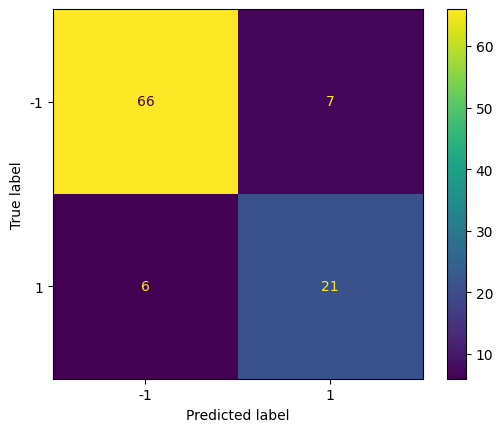
Compute the classification accuracy on the test set.
clf.best_estimator_.score(X_test, y_test)
0.87
This is the accuracy of the best model on the test set.
8.3.3.2. Evaluation via ROC curves
Now, let us compare the ROC curves of two models on the training/test data with different hyperparameter \(\gamma\) of RBF kernel. Set probability=True in the SVC constructor if you would like to have the class probability output. Read the docs on scores and probabilities of scikit-learn for more details.
Let us use a lightly larger value of gamma for the first model to compare.
svm3 = SVC(C=1, kernel="rbf", gamma=2, probability=True)
svm3.fit(X_train, y_train)
SVC(C=1, gamma=2, probability=True)In a Jupyter environment, please rerun this cell to show the HTML representation or trust the notebook.
On GitHub, the HTML representation is unable to render, please try loading this page with nbviewer.org.
SVC(C=1, gamma=2, probability=True)
Let us use a larger value of gamma for the second model to compare. This will result in a more flexible decision boundary, and will likely overfit the data more.
svm4 = SVC(C=1, kernel="rbf", gamma=50, probability=True)
svm4.fit(X_train, y_train)
SVC(C=1, gamma=50, probability=True)In a Jupyter environment, please rerun this cell to show the HTML representation or trust the notebook.
On GitHub, the HTML representation is unable to render, please try loading this page with nbviewer.org.
SVC(C=1, gamma=50, probability=True)
Let us plot the ROC curves of the two models on the training dataset and then on the test dataset.
y_train_score3 = svm3.decision_function(X_train)
y_train_score4 = svm4.decision_function(X_train)
# comment the above two lines uncomment the following two lines to plot the ROC curves using probabilities
# y_train_score3 = svm3.predict_proba(X_train)[:, 1]
# y_train_score4 = svm4.predict_proba(X_train)[:, 1]

false_pos_rate3, true_pos_rate3, _ = roc_curve(y_train, y_train_score3)
roc_auc3 = auc(false_pos_rate3, true_pos_rate3)

false_pos_rate4, true_pos_rate4, _ = roc_curve(y_train, y_train_score4)
roc_auc4 = auc(false_pos_rate4, true_pos_rate4)

fig, (ax1, ax2) = plt.subplots(1, 2, figsize=(14, 6))
ax1.plot(
    false_pos_rate3,
    true_pos_rate3,
    label="SVM $\gamma = 1$ ROC curve (area = %0.2f)" % roc_auc3,
    color="b",
)
ax1.plot(
    false_pos_rate4,
    true_pos_rate4,
    label="SVM $\gamma = 50$ ROC curve (area = %0.2f)" % roc_auc4,
    color="r",
)
ax1.set_title("Training Data")

y_test_score3 = svm3.decision_function(X_test)
y_test_score4 = svm4.decision_function(X_test)
# comment the above two lines uncomment the following two lines to plot the ROC curves using probabilities
# y_test_score3 = svm3.predict_proba(X_test)[:, 1]
# y_test_score4 = svm4.predict_proba(X_test)[:, 1]

false_pos_rate3, true_pos_rate3, _ = roc_curve(y_test, y_test_score3)
roc_auc3 = auc(false_pos_rate3, true_pos_rate3)

false_pos_rate4, true_pos_rate4, _ = roc_curve(y_test, y_test_score4)
roc_auc4 = auc(false_pos_rate4, true_pos_rate4)

ax2.plot(
    false_pos_rate3,
    true_pos_rate3,
    label="SVM $\gamma = 1$ ROC curve (area = %0.2f)" % roc_auc3,
    color="b",
)
ax2.plot(
    false_pos_rate4,
    true_pos_rate4,
    label="SVM $\gamma = 50$ ROC curve (area = %0.2f)" % roc_auc4,
    color="r",
)
ax2.set_title("Test Data")

for ax in fig.axes:
    ax.plot([0, 1], [0, 1], "k--")
    ax.set_xlim([-0.05, 1.0])
    ax.set_ylim([0.0, 1.05])
    ax.set_xlabel("False Positive Rate")
    ax.set_ylabel("True Positive Rate")
    ax.legend(loc="lower right")
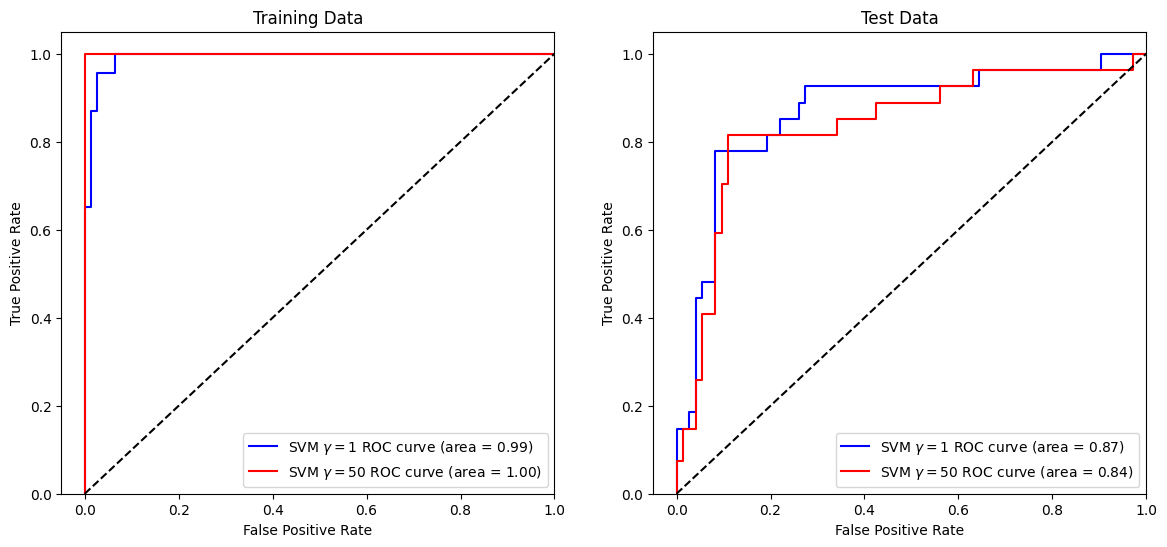
As we can see from the above, the more flexible model (with \( \gamma = 50 \)) scores better (perfectly) on the training dataset but worse on the test dataset.
8.3.4. SVM with more than two classes
So far, our discussion has been limited to the case of binary classification, i.e. the two-class setting. How can we extend SVM (or logistic regression) to the more general case where we have some arbitrary number of classes? It turns out that the concept of separating hyperplanes upon which SVMs are based does not lend itself naturally to more than two classes. There are multiple ways to extend SVMs to the multi-class settings. The two most popular solutions are the one-versus-one and one-versus-all approaches.
8.3.4.1. One-vs-one
Suppose that we would like to perform classification using SVMs, and there are \(C\) > 2 classes. A one-versus-one or all-pairs approach constructs \(C(C-1)/2\) binary classifiers, one for each pair of classes. For example, if there are three classes, then we would construct three binary classifiers, one for each pair of classes. The first classifier would distinguish between class 1 and class 2, the second classifier would distinguish between class 1 and class 3, and the third classifier would distinguish between class 2 and class 3. To classify a new observation, we would apply each of the three classifiers, and assign the observation to the class that receives the most votes.
8.3.4.2. One-vs-all
The one-versus-all approach is an alternative procedure for applying SVMs in the case of \(C\) > 2 classes. We fit \(C\) SVMs, each time comparing one of the \(C\) classes to the remaining \(C − 1\) classes. For example, if there are three classes, then we would fit three SVMs, one for each class. The first SVM would separate class 1 from classes 2 and 3, the second SVM would separate class 2 from classes 1 and 3, and the third SVM would separate class 3 from classes 1 and 2. To classify a new observation, we would apply each of these three classifiers, and assign the observation to the class that receives the most votes.
The following code shows how to train a multi-class SVM using scikit-learn. The strategy for multi-class classification is “one vs one” internally. However, we can get “one vs rest” hyperplane by setting decision_function_shape='ovr' in the SVC object.
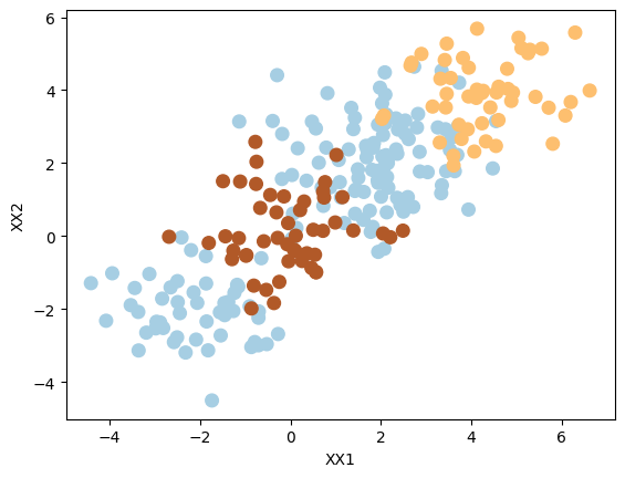
Add a third class of observations
XX = np.vstack([X, np.random.randn(50, 2)])
yy = np.hstack([y, np.repeat(0, 50)])
XX[yy == 0] = XX[yy == 0] + 4

plt.scatter(XX[:, 0], XX[:, 1], s=70, c=yy, cmap=plt.cm.Paired)
plt.xlabel("XX1")
plt.ylabel("XX2");
Use SVM with an RBF kernel to fit a three-class classifier and plot the decision boundaries.
svm5 = SVC(C=1, kernel="rbf")
svm5.fit(XX, yy)
plot_svc(svm5, XX, yy)
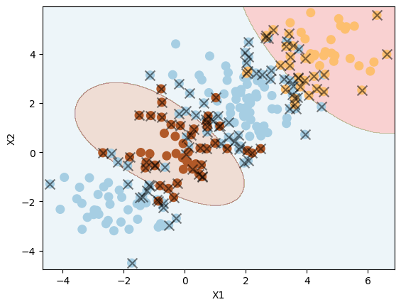
Number of support vectors: 125
We can see the classifying three classes (in 2D) is not easy, as expected.
8.3.5. Exercises
1. All the following exercises use the Heart dataset.
Load the Heart dataset, convert the values of variables (predictors) from categorical values to numerical values, and inspect the first five rows.
# Write your code below to answer the question
Compare your answer with the reference solution below
import numpy as np
import pandas as pd

np.random.seed(2022)

heart_url = "https://github.com/pykale/transparentML/raw/main/data/Heart.csv"

heart_df = pd.read_csv(heart_url, index_col=0).dropna()
# converting categories
heart_df["ChestPain"] = heart_df["ChestPain"].factorize()[0]
heart_df["Thal"] = heart_df["Thal"].factorize()[0]
heart_df["AHD"] = heart_df["AHD"].factorize()[0]

heart_df.head(5)
| Age | Sex | ChestPain | RestBP | Chol | Fbs | RestECG | MaxHR | ExAng | Oldpeak | Slope | Ca | Thal | AHD | |
|---|---|---|---|---|---|---|---|---|---|---|---|---|---|---|
| 1 | 63 | 1 | 0 | 145 | 233 | 1 | 2 | 150 | 0 | 2.3 | 3 | 0.0 | 0 | 0 |
| 2 | 67 | 1 | 1 | 160 | 286 | 0 | 2 | 108 | 1 | 1.5 | 2 | 3.0 | 1 | 1 |
| 3 | 67 | 1 | 1 | 120 | 229 | 0 | 2 | 129 | 1 | 2.6 | 2 | 2.0 | 2 | 1 |
| 4 | 37 | 1 | 2 | 130 | 250 | 0 | 0 | 187 | 0 | 3.5 | 3 | 0.0 | 1 | 0 |
| 5 | 41 | 0 | 3 | 130 | 204 | 0 | 2 | 172 | 0 | 1.4 | 1 | 0.0 | 1 | 0 |
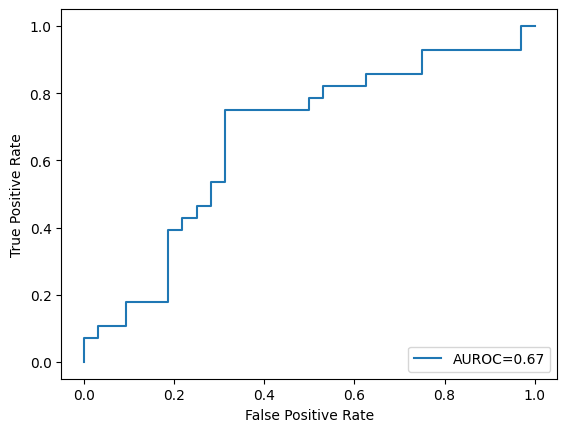
2. Split the loaded dataset into training and testing sets in an \(80:20\) ratio, then train a model using SVC using these hyperparameters: C = 1, kernel = “rbf, gamma = 0.01, probability = true. Here, kernel =”rbf” means we are using the RBF kernel to increase the dimensionality of the feature space, extending SVC into an SVM. Finally, show the number of support vectors and plot the AUROC curve of this trained model on the test set. (Use \(2022\) as the random seed value)
# Write your code below to answer the question
Compare your answer with the reference solution below
from sklearn.svm import SVC
from sklearn.model_selection import train_test_split
from sklearn.metrics import roc_curve, auc
import matplotlib.pyplot as plt

np.random.seed(2022)

X = heart_df.drop(["AHD"], axis=1)
y = heart_df["AHD"]


X_train, X_test, y_train, y_test = train_test_split(
    X, y.ravel(), test_size=0.2, random_state=2022
)

svm = SVC(C=1, kernel="rbf", gamma=0.01, probability=True, random_state=2022)
svm.fit(X_train, y_train)
print("Number of Support vectors: ", len(svm.support_vectors_))

y_test_score = svm.decision_function(X_test)

fpr, tpr, _ = roc_curve(y_test, y_test_score)
roc_auc = auc(fpr, tpr)

plt.plot(fpr, tpr, label="AUROC=" + str(np.round(roc_auc, 2)))
plt.ylabel("True Positive Rate")
plt.xlabel("False Positive Rate")
plt.legend(loc=4)
plt.show()
Number of Support vectors: 234
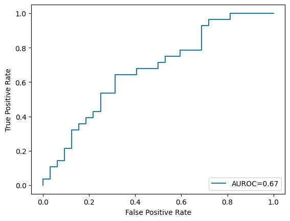
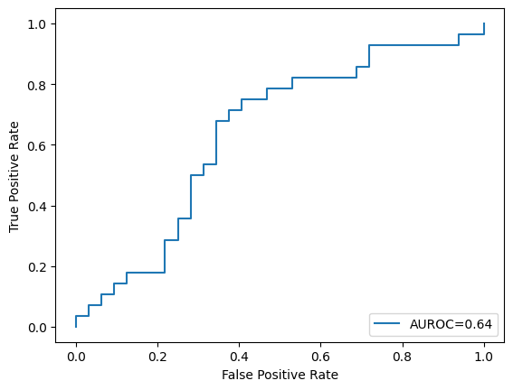
3. Train another model in the same manner as in Exercise 2, but with the hyperparameter regularisation strength \(C\) set to \(100\). Show the number of support vectors and plot the AUROC curve of this trained model on the test set.
# Write your code below to answer the question
Compare your answer with the reference solution below
svm = SVC(C=100, kernel="rbf", gamma=0.01, probability=True, random_state=2022)
svm.fit(X_train, y_train)
print("Number of Support vectors: ", len(svm.support_vectors_))

y_test_score = svm.decision_function(X_test)

fpr, tpr, _ = roc_curve(y_test, y_test_score)
roc_auc = auc(fpr, tpr)

plt.plot(fpr, tpr, label="AUROC=" + str(np.round(roc_auc, 2)))
plt.ylabel("True Positive Rate")
plt.xlabel("False Positive Rate")
plt.legend(loc=4)
plt.show()
Number of Support vectors: 233
4. Using GridSearchCV, fine-tune the SVM hyperparameters (\(C\) and \(gamma\)) on the training dataset (using \(10\)-fold cross-validation) for \(C\) values of \(0.001\), \(0.01\), \(0.1\), \(5\) and \(gamma\) values of \(0.001\), \(0.01\), \(0.1\), \(0.5\), \(1\). Display the best hyperparameters value for \(C\) and \(gamma\). (Use the roc_auc scoring for choosing the best model and its hyperparameters).
# Write your code below to answer the question
Compare your answer with the reference solution below
from sklearn.model_selection import GridSearchCV

tuned_parameters = {"C": [0.01, 0.1, 1, 10, 100], "gamma": [0.001, 0.01, 0.1, 0.5, 1]}
clf = GridSearchCV(
    SVC(kernel="rbf", probability=True, random_state=2022),
    tuned_parameters,
    cv=10,
    scoring="roc_auc",
    return_train_score=True,
)
clf.fit(X_train, y_train)
print("\nOptimal parameters : ", clf.best_params_)
Optimal parameters : {'C': 1, 'gamma': 0.001}
5. Finally, using the best hyperparameters from Exercise 4, train another SVM model on the training dataset and plot the AUROC curve of this trained model on the test set.
# Write your code below to answer the question
Compare your answer with the reference solution below
svm = SVC(C=1, kernel="rbf", gamma=0.001, probability=True, random_state=2022)
svm.fit(X_train, y_train)
print("Number of Support vectors: ", len(svm.support_vectors_))

y_test_score = svm.decision_function(X_test)

fpr, tpr, _ = roc_curve(y_test, y_test_score)
roc_auc = auc(fpr, tpr)

plt.plot(fpr, tpr, label="AUROC=" + str(np.round(roc_auc, 2)))
plt.ylabel("True Positive Rate")
plt.xlabel("False Positive Rate")
plt.legend(loc=4)
plt.show()
Number of Support vectors: 189