Extensions/limitations of linear regression
Contents
2.3. Extensions/limitations of linear regression
Read then Launch
This content is best viewed in html because jupyter notebook cannot display some content (e.g. figures, equations) properly. You should finish reading this page first and then launch it as an interactive notebook in Google Colab (faster, Google account needed) or Binder by clicking the rocket symbol () at the top.
This section studies how to extend linear regression to more complicated types of variables and relationships, and the limitations of linear regression. We will use three datasets to illustrate these concepts:
The Advertising dataset that has been used in the previous sections.
The Credit dataset contains information about credit card holders. The goal is to predict the credit
Limitfor each card holder.The Auto dataset dataset contains information about the characteristics of cars. The goal is to predict the
mpg(miles per gallon) for a car based on its features likehorsepower,weightandacceleration. This dataset has also been used in the tutorial of Prerequisites.
You are encouraged to click the links to the datasets and explore the variables and understand their relationships.
2.3.1. Import libraries and load data
Get ready by importing the APIs needed from respective libraries.
import pandas as pd
import numpy as np
import matplotlib.pyplot as plt
import seaborn as sns

from sklearn.preprocessing import scale
from sklearn.linear_model import LinearRegression

from statsmodels.formula.api import ols

%matplotlib inline
Load the Advertising dataset dataset that we are already familiar with.
data_url = "https://github.com/pykale/transparentML/raw/main/data/Advertising.csv"
advertising_df = pd.read_csv(data_url, header=0, index_col=0)
Load the Credit dataset dataset, convert the Student2 category to numbers (‘0’ and ‘1’), and inspect the first three rows.
credit_url = "https://github.com/pykale/transparentML/raw/main/data/Credit.csv"

credit_df = pd.read_csv(credit_url)
credit_df["Student2"] = credit_df.Student.map({"No": 0, "Yes": 1})
credit_df.head(3)
| Income | Limit | Rating | Cards | Age | Education | Own | Student | Married | Region | Balance | Student2 | |
|---|---|---|---|---|---|---|---|---|---|---|---|---|
| 0 | 14.891 | 3606 | 283 | 2 | 34 | 11 | No | No | Yes | South | 333 | 0 |
| 1 | 106.025 | 6645 | 483 | 3 | 82 | 15 | Yes | Yes | Yes | West | 903 | 1 |
| 2 | 104.593 | 7075 | 514 | 4 | 71 | 11 | No | No | No | West | 580 | 0 |
Load the Auto dataset datasets, ignore rows with missing values, and inspect the columns, counts and data types.
auto_url = "https://github.com/pykale/transparentML/raw/main/data/Auto.csv"

auto_df = pd.read_csv(auto_url, na_values="?").dropna()
auto_df.info()
<class 'pandas.core.frame.DataFrame'>
Index: 392 entries, 0 to 396
Data columns (total 9 columns):
 #   Column        Non-Null Count  Dtype
---  ------        --------------  -----
 0   mpg           392 non-null    float64
 1   cylinders     392 non-null    int64
 2   displacement  392 non-null    float64
 3   horsepower    392 non-null    float64
 4   weight        392 non-null    int64
 5   acceleration  392 non-null    float64
 6   year          392 non-null    int64
 7   origin        392 non-null    int64
 8   name          392 non-null    object
dtypes: float64(4), int64(4), object(1)
memory usage: 30.6+ KB
2.3.2. Qualitative predictors
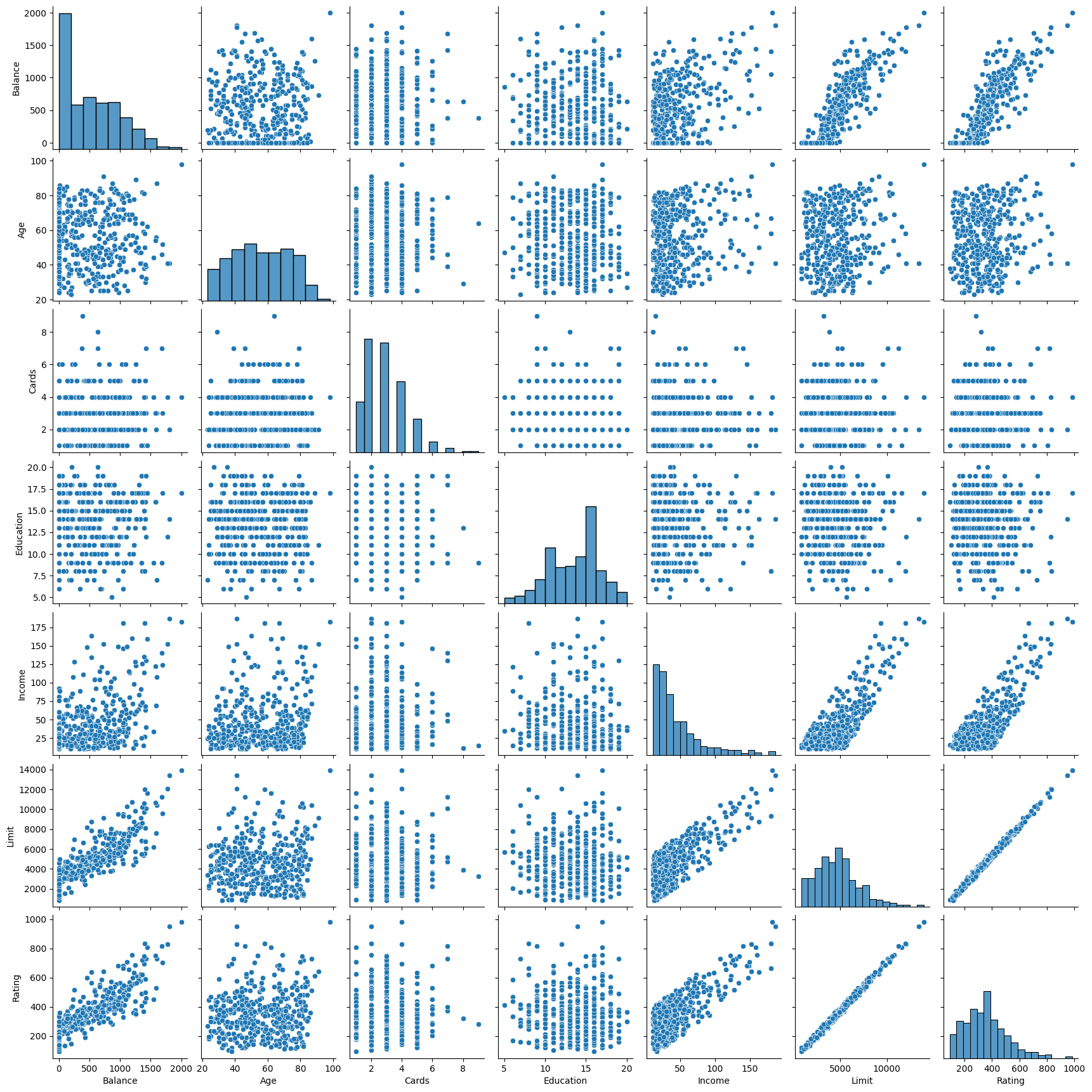
In the previous sections, the predictor variables are quantitative. Here, in the Credit dataset, the response is Balance (average credit card debt for each individual) and there are six quantitative predictors: Age , Cards (number of credit cards), Education (years of education), Income (in thousands of dollars), Limit (credit limit), and Rating (credit rating). The following code displays the pairwise relationships between these variables (Figure 3.6 in the textbook).
sns.pairplot(
    credit_df[["Balance", "Age", "Cards", "Education", "Income", "Limit", "Rating"]]
)
plt.show()
However, in practice, predictor variables are not always quantitative. For example, in the Credit dataset, it also contains four qualitative (categorical) variables: Student (Yes or No), Own (Yes or No), Married (Yes or No), and Region (South, East, or West).
Predictors with only two levels
If a qualitative predictor has only two levels (possible values), then we can treat it as a quantitative variable, known as an indicator or dummy variable. For example, the Student variable has two levels: Yes and No. We can convert these levels to numbers, such as 1 and 0, and then treat the Student variable as a quantitative variable. This is called coding the qualitative variable, which is automatically done by the statsmodels library.
Run the following code to get the least squares coefficient estimates associated with the regression of Balance onto Own in the Credit dataset (Table 3.7 in the textbook).
est = ols("Balance ~ Own", credit_df).fit()
est.summary().tables[1]
| coef | std err | t | P>|t| | [0.025 | 0.975] | |
|---|---|---|---|---|---|---|
| Intercept | 509.8031 | 33.128 | 15.389 | 0.000 | 444.675 | 574.931 |
| Own[T.Yes] | 19.7331 | 46.051 | 0.429 | 0.669 | -70.801 | 110.267 |
The large \(p\) value above shows that there is no relationship between Balance and Own.
Predictors with more than two levels
When a qualitative predictor has more than two levels, we need to create additional dummy variables. For example, the Region variable has three levels: South, East, and West. We can create two dummy variables, South, and West, and then use these variables in the regression model. There will be always one fewer dummy variable than the number of levels in the qualitative variable. This is because the regression model can determine the value of the missing dummy variable. For example, if South is 0 and West is 0, then the individual must be from the East region. Again, such coding is automatically done by the statsmodels library.
Run the following code to get the least squares coefficient estimates associated with the regression of Balance onto Region in the Credit dataset (Table 3.8 in the textbook).
est = ols("Balance ~ Region", credit_df).fit()
est.summary().tables[1]
| coef | std err | t | P>|t| | [0.025 | 0.975] | |
|---|---|---|---|---|---|---|
| Intercept | 531.0000 | 46.319 | 11.464 | 0.000 | 439.939 | 622.061 |
| Region[T.South] | -12.5025 | 56.681 | -0.221 | 0.826 | -123.935 | 98.930 |
| Region[T.West] | -18.6863 | 65.021 | -0.287 | 0.774 | -146.515 | 109.142 |
The large \(p\)-values above show that there is no relationship between Balance and Region.
2.3.3. Extensions of linear regression
2.3.3.1. Interaction between variables
In the previous analysis of Advertising dataset, the predictor variables are assumed to be independent. However, this model may be incorrect. For example, radio advertising can increase the effectiveness of TV advertising, which is known as interaction effect in statistics. Consider the standard multiple linear regression with two variables
This model can be extended to include an interaction term between \(x_1\) and \(x_2\):
where \(\tilde{\beta}_1 = \beta_1 + \beta_3 x_2\) is the effective coefficient on \(x_1\), which can be viewed as another linear regression that regresses \(\tilde{\beta}_1\) onto \(x_2\). Then the association between \(y\) and \(x_1\) is no longer constant and depends on the value of \(x_2\). Similarly, the association between \(y\) and \(x_2\) is no longer constant and depends on the value of \(x_1\).
Run the following code for the Advertising data to get the least squares coefficient estimates associated with the regression of Sales onto TV and Radio, with an interaction term, TV \(\times\) Radio (Table 3.9 of the text book).
est = ols("Sales ~ TV + Radio + TV*Radio", advertising_df).fit()
est.summary().tables[1]
| coef | std err | t | P>|t| | [0.025 | 0.975] | |
|---|---|---|---|---|---|---|
| Intercept | 6.7502 | 0.248 | 27.233 | 0.000 | 6.261 | 7.239 |
| TV | 0.0191 | 0.002 | 12.699 | 0.000 | 0.016 | 0.022 |
| Radio | 0.0289 | 0.009 | 3.241 | 0.001 | 0.011 | 0.046 |
| TV:Radio | 0.0011 | 5.24e-05 | 20.727 | 0.000 | 0.001 | 0.001 |
The small \(p\)-value for the interaction term suggests that the true relationship is not additive and there is strong evidence of the association between Sales and the interaction between TV and Radio. Without including the interaction term, our understanding of the relationship between Sales and TV and Radio is not complete.
2.3.3.1.1. Interaction between qualitative and quantitative variables
The concept of interactions also applies to qualitative variables. In fact, sometimes an interaction between a qualitative variable and a quantitative variable has a particularly nice interpretation. For example, run the following code to predict Balance using the Income (quantitative) and Student (qualitative) variables, and compare the differences between including and excluding the interaction term between Income and Student.
est1 = ols("Balance ~ Income + Student2", credit_df).fit()
est2 = ols("Balance ~ Income + Income*Student2", credit_df).fit()

print("Regression 1 - without interaction term")
print(est1.params)
print("\nRegression 2 - with interaction term")
print(est2.params)
Regression 1 - without interaction term
Intercept    211.142964
Income         5.984336
Student2     382.670539
dtype: float64

Regression 2 - with interaction term
Intercept          200.623153
Income               6.218169
Student2           476.675843
Income:Student2     -1.999151
dtype: float64
We can see that the interaction term between Income and Student affects the relationship between Balance and Student more than the relationship between Balance and Income. To have a closer look, let us visualise the relationship between Balance and Income for students and non-students separately (Figure 3.7 of the textbook).
# Income (x-axis)
regr1 = est1.params
regr2 = est2.params

income = np.linspace(0, 150)

# Balance without interaction term (y-axis)
student1 = np.linspace(
    regr1["Intercept"] + regr1["Student2"],
    regr1["Intercept"] + regr1["Student2"] + 150 * regr1["Income"],
)
non_student1 = np.linspace(
    regr1["Intercept"], regr1["Intercept"] + 150 * regr1["Income"]
)

# Balance with interaction term (y-axis)
student2 = np.linspace(
    regr2["Intercept"] + regr2["Student2"],
    regr2["Intercept"]
    + regr2["Student2"]
    + 150 * (regr2["Income"] + regr2["Income:Student2"]),
)
non_student2 = np.linspace(
    regr2["Intercept"], regr2["Intercept"] + 150 * regr2["Income"]
)

# Create plot
fig, (ax1, ax2) = plt.subplots(1, 2, figsize=(12, 5))
ax1.plot(income, student1, "r-", income, non_student1, "k-")
ax2.plot(income, student2, "r--", income, non_student2, "k--")

for ax in fig.axes:
    ax.legend(["student", "non-student"], loc=2)
    ax.set_xlabel("Income")
    ax.set_ylabel("Balance")
    ax.set_ylim(ymax=1550)
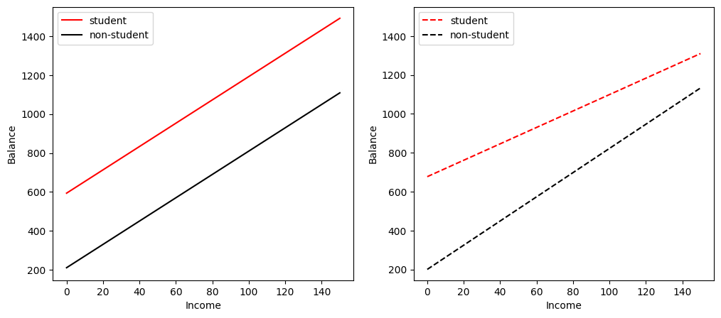
In the left figure without the interaction term between Income and Student, we see two (solid) parallel lines, one for students and one for non-students. The two lines have different intercepts but the same slope, indicating that a one-unit increase in Income will have the same effect on Balance for students and non-students, which is counterintuitive.
In the right figure with the interaction term between Income and Student, the two (dashed) lines are no longer parallel. We see that the slope of the line for students is flatter than that for non-students, indicating that a one-unit increase in Income will have a much smaller effect on credit card Balance for students than for non-students. This is consistent with our intuition.
2.3.3.2. Nonlinear relationships
In some cases, the true relationship between the response and the predictors may be nonlinear. Here we present a very simple way to directly extend the linear model to accommodate nonlinear relationships, using polynomial regression.
Run the following code to observe the relationship between mpg (gas mileage in miles per gallon) and horsepower.
plt.scatter(
    auto_df.horsepower, auto_df.mpg, facecolors="None", edgecolors="k", alpha=0.5
)
plt.xlabel("horsepower")
plt.ylabel("mpg")
Text(0, 0.5, 'mpg')
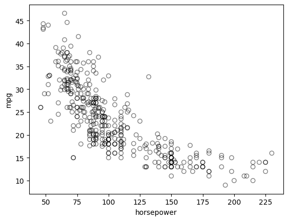
The figure shows a strong relationship between mpg and horsepower, but it is clearly not linear. We can use a polynomial regression to fit a nonlinear model to the data. We can fit a polynomial regression of degree 2 (quadratic) to the data using the following regression:
Run the following code to display the relationship between mpg (gas mileage in miles per gallon) and \(\textrm{horsepower}^2\) as well as \(\textrm{horsepower}^5\) (Figure 3.8 of the textbook) for cars in the Auto dataset.
# With Seaborn's regplot() you can easily plot higher order polynomials.
plt.scatter(
    auto_df.horsepower, auto_df.mpg, facecolors="None", edgecolors="k", alpha=0.5
)

sns.regplot(
    x=auto_df.horsepower,
    y=auto_df.mpg,
    ci=None,
    label="Linear",
    scatter=False,
    color="orange",
)
sns.regplot(
    x=auto_df.horsepower,
    y=auto_df.mpg,
    ci=None,
    label="Degree 2",
    order=2,
    scatter=False,
    color="lightblue",
)
sns.regplot(
    x=auto_df.horsepower,
    y=auto_df.mpg,
    ci=None,
    label="Degree 5",
    order=5,
    scatter=False,
    color="g",
)
plt.legend()
plt.ylim(5, 55)
plt.xlim(40, 240);
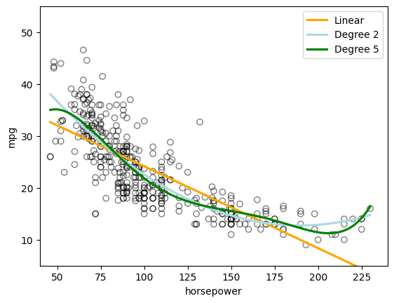
The above figure seems to suggest that a quadratic relationship between mpg and horsepower is more appropriate than a linear relationship.
In fact, this is still a linear model with \(x_1 = \textrm{horsepower}\) and \(x_2 = \textrm{horsepower}^2\). Run the following code to create a new predictor horsepower2 and inspect the Auto dataset.
auto_df["horsepower2"] = auto_df.horsepower**2
auto_df.head(3)
| mpg | cylinders | displacement | horsepower | weight | acceleration | year | origin | name | horsepower2 | |
|---|---|---|---|---|---|---|---|---|---|---|
| 0 | 18.0 | 8 | 307.0 | 130.0 | 3504 | 12.0 | 70 | 1 | chevrolet chevelle malibu | 16900.0 |
| 1 | 15.0 | 8 | 350.0 | 165.0 | 3693 | 11.5 | 70 | 1 | buick skylark 320 | 27225.0 |
| 2 | 18.0 | 8 | 318.0 | 150.0 | 3436 | 11.0 | 70 | 1 | plymouth satellite | 22500.0 |
Then run the following code to fit a linear regression model with mpg as the response and horsepower and horsepower2 as the predictors (Table 3.10 of the textbook).
est = ols("mpg ~ horsepower + horsepower2", auto_df).fit()
est.summary().tables[1]
| coef | std err | t | P>|t| | [0.025 | 0.975] | |
|---|---|---|---|---|---|---|
| Intercept | 56.9001 | 1.800 | 31.604 | 0.000 | 53.360 | 60.440 |
| horsepower | -0.4662 | 0.031 | -14.978 | 0.000 | -0.527 | -0.405 |
| horsepower2 | 0.0012 | 0.000 | 10.080 | 0.000 | 0.001 | 0.001 |
2.3.3.3. Limitations of linear regression
Every model will have some limitations, and linear regression is no exception. Here we briefly study two of the limitations of linear regression to show the possible complexities of real-world data. More limitations can be found in the textbook.
2.3.3.3.1. Nonlinearity of the Data
The linear regression model assumes that there is a “straight-line” relationship between the predictors and the response. If the true relationship is far from linear, then virtually all of the conclusions that we draw from the fit are questionable. In addition, the prediction accuracy of the model can be significantly reduced.
Run the following code to compare the differences in accuracy between a linear regression model and a quadratic regression model for regressing mpg onto horsepower.
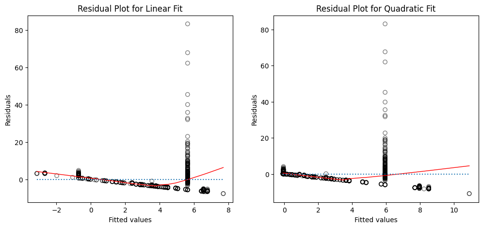
Firstly, fitting a linear regression model and a quadratic regression model for regressing mpg onto horsepower and compute the residuals for each model.
regr = LinearRegression()

# Linear fit
X = auto_df.horsepower.values.reshape(-1, 1)
y = auto_df.mpg
regr.fit(X, y)

auto_df["pred1"] = regr.predict(X)
auto_df["resid1"] = auto_df.mpg - auto_df.pred1

# Quadratic fit
X2 = auto_df[["horsepower", "horsepower2"]].values
regr.fit(X2, y)

auto_df["pred2"] = regr.predict(X2)
auto_df["resid2"] = auto_df.mpg - auto_df.pred2
Create plots of the residuals for each model. What do you observe?
fig, (ax1, ax2) = plt.subplots(1, 2, figsize=(12, 5))

# Left plot
sns.regplot(
    x=auto_df.pred1,
    y=auto_df.resid1,
    lowess=True,
    ax=ax1,
    line_kws={"color": "r", "lw": 1},
    scatter_kws={"facecolors": "None", "edgecolors": "k", "alpha": 0.5},
)
ax1.hlines(
    0,
    xmin=ax1.xaxis.get_data_interval()[0],
    xmax=ax1.xaxis.get_data_interval()[1],
    linestyles="dotted",
)
ax1.set_title("Residual Plot for Linear Fit")

# Right plot
sns.regplot(
    x=auto_df.pred2,
    y=auto_df.resid2,
    lowess=True,
    line_kws={"color": "r", "lw": 1},
    ax=ax2,
    scatter_kws={"facecolors": "None", "edgecolors": "k", "alpha": 0.5},
)
ax2.hlines(
    0,
    xmin=ax2.xaxis.get_data_interval()[0],
    xmax=ax2.xaxis.get_data_interval()[1],
    linestyles="dotted",
)
ax2.set_title("Residual Plot for Quadratic Fit")

for ax in fig.axes:
    ax.set_xlabel("Fitted values")
    ax.set_ylabel("Residuals")
How to interpret the plots?
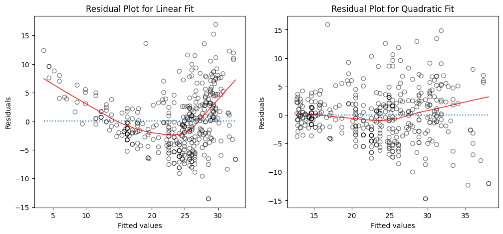
The left panel displays a residual plot from the linear regression of
mpgontohorsepoweron theAutodataset. The red line is a smooth fit to the residuals for identifying any trends in the residuals. Here, the residuals exhibit a clear U-shape, which provides a strong indication of nonlinearity in the data.The right panel displays the residual plot that results from the model contains a quadratic term. There appears to be little pattern in the residuals, suggesting that the quadratic term improves the fit to the data.
2.3.3.4. Collinearity
Collinearity refers to the situation in which two or more predictor variables are closely related to one another.
Run the following code to illustrate the problem of collinearity in the Credit dataset (Figure 3.14 of the textbook).
fig, (ax1, ax2) = plt.subplots(1, 2, figsize=(12, 5))

# Left plot
ax1.scatter(credit_df.Limit, credit_df.Age, facecolor="None", edgecolor="r")
ax1.set_ylabel("Age")

# Right plot
ax2.scatter(credit_df.Limit, credit_df.Rating, facecolor="None", edgecolor="r")
ax2.set_ylabel("Rating")

for ax in fig.axes:
    ax.set_xlabel("Limit")
    ax.set_xticks([2000, 4000, 6000, 8000, 12000])
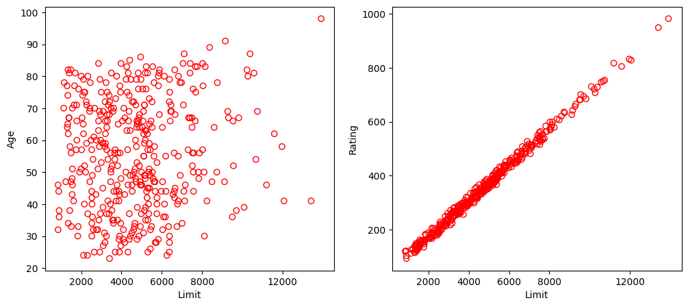
In the left panel, the two predictors limit and age appear to have no obvious relationship. In contrast, in the right panel, the predictors limit and rating are very highly correlated with each other, and we say that they are collinear. In this context, limit and rating tend to increase or decrease together, it can be difficult to determine how each one separately is associated with the response balance.
Run the following code to learn the difficulties that can result from collinearity in the context of the Credit dataset.
y = credit_df.Balance

# Regression for left plot
X = credit_df[["Age", "Limit"]].values
regr1 = LinearRegression()
regr1.fit(scale(X.astype("float"), with_std=False), y)
print("Age/Limit\n", regr1.intercept_)
print(regr1.coef_)

# Regression for right plot
X2 = credit_df[["Rating", "Limit"]].values
regr2 = LinearRegression()
regr2.fit(scale(X2.astype("float"), with_std=False), y)
print("\nRating/Limit\n", regr2.intercept_)
print(regr2.coef_)
Age/Limit
 520.0150000000001
[-2.29148553  0.17336497]

Rating/Limit
 520.015
[2.20167217 0.02451438]
Create grid coordinates for plotting and then calculate RSS based on grid of coefficients
# grid coordinates
beta_age = np.linspace(regr1.coef_[0] - 3, regr1.coef_[0] + 3, 100)
beta_limit = np.linspace(regr1.coef_[1] - 0.02, regr1.coef_[1] + 0.02, 100)

beta_rating = np.linspace(regr2.coef_[0] - 3, regr2.coef_[0] + 3, 100)
beta_limit2 = np.linspace(regr2.coef_[1] - 0.2, regr2.coef_[1] + 0.2, 100)

X1, Y1 = np.meshgrid(beta_limit, beta_age, indexing="xy")
X2, Y2 = np.meshgrid(beta_limit2, beta_rating, indexing="xy")
Z1 = np.zeros((beta_age.size, beta_limit.size))
Z2 = np.zeros((beta_rating.size, beta_limit2.size))

limit_scaled = scale(credit_df.Limit.astype("float"), with_std=False)
age_scaled = scale(credit_df.Age.astype("float"), with_std=False)
rating_scaled = scale(credit_df.Rating.astype("float"), with_std=False)

# calculate RSS
for (i, j), v in np.ndenumerate(Z1):
    Z1[i, j] = (
        (y - (regr1.intercept_ + X1[i, j] * limit_scaled + Y1[i, j] * age_scaled)) ** 2
    ).sum() / 1000000

for (i, j), v in np.ndenumerate(Z2):
    Z2[i, j] = (
        (y - (regr2.intercept_ + X2[i, j] * limit_scaled + Y2[i, j] * rating_scaled))
        ** 2
    ).sum() / 1000000
Plot the contours of the RSS with respect to the coefficients of the two linear regression models in 2D.
from matplotlib.pyplot import contour


fig = plt.figure(figsize=(12, 5))
fig.suptitle("RSS - Regression coefficients", fontsize=20)

ax1 = fig.add_subplot(121)
ax2 = fig.add_subplot(122)

min_RSS = r"$\beta_0$, $\beta_1$ for minimized RSS"

# Left plot
contour1 = ax1.contour(X1, Y1, Z1, cmap=plt.cm.Set1, levels=[21.25, 21.5, 21.8])
ax1.scatter(regr1.coef_[1], regr1.coef_[0], c="r", label=min_RSS)
ax1.clabel(contour1, inline=True, fontsize=10, fmt="%1.1f")
ax1.set_ylabel(r"$\beta_{Age}$", fontsize=17)

# Right plot
contour2 = ax2.contour(X2, Y2, Z2, cmap=plt.cm.Set1, levels=[21.5, 21.8])
ax2.scatter(regr2.coef_[1], regr2.coef_[0], c="r", label=min_RSS)
ax2.clabel(contour2, inline=True, fontsize=10, fmt="%1.1f")
ax2.set_ylabel(r"$\beta_{Rating}$", fontsize=17)
ax2.set_xticks([-0.1, 0, 0.1, 0.2])

for ax in fig.axes:
    ax.set_xlabel(r"$\beta_{Limit}$", fontsize=17)
    ax.legend()
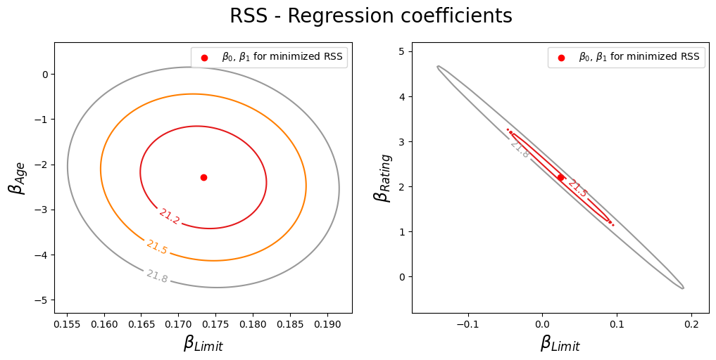
Left: A contour plot of RSS for the regression of balance onto age and limit. The minimum value is well defined.
Right: A contour plot of RSS for the regression of balance onto rating and limit. Because of the collinearity, there are many pairs (\(\beta_{\text{Limit}}\) , \(\beta_{\text{Rating}}\)) with a similar value for RSS.
Collinearity reduces the accuracy of the estimates of the regression coefficients, it causes the standard error for \(\hat{\beta}_j\) to grow. In the presence of collinearity, we may fail to reject \(H_0\) : \(\hat{\beta}_j = 0\). This means that the power of the hypothesis test—the probability of correctly detecting a non-zero coefficient is reduced by collinearity.
Run the following code to compare the coefficient estimates obtained from two separate multiple regression models using statsmodels, where the first model is a regression of balance on age and limit, and the second model is a regression of balance on rating and limit.
est_age_limit = ols("Balance ~ Age + Limit", credit_df).fit()
est_age_limit.summary().tables[1]
| coef | std err | t | P>|t| | [0.025 | 0.975] | |
|---|---|---|---|---|---|---|
| Intercept | -173.4109 | 43.828 | -3.957 | 0.000 | -259.576 | -87.246 |
| Age | -2.2915 | 0.672 | -3.407 | 0.001 | -3.614 | -0.969 |
| Limit | 0.1734 | 0.005 | 34.496 | 0.000 | 0.163 | 0.183 |
est_rating_limit = ols("Balance ~ Rating + Limit", credit_df).fit()
est_rating_limit.summary().tables[1]
| coef | std err | t | P>|t| | [0.025 | 0.975] | |
|---|---|---|---|---|---|---|
| Intercept | -377.5368 | 45.254 | -8.343 | 0.000 | -466.505 | -288.569 |
| Rating | 2.2017 | 0.952 | 2.312 | 0.021 | 0.330 | 4.074 |
| Limit | 0.0245 | 0.064 | 0.384 | 0.701 | -0.101 | 0.150 |
The above generates Table 3.11 of the textbook.
How to interpret the results?
In the first regression, both age and limit are highly significant with very small \(p\)-values. In the second, the collinearity between limit and rating has caused the standard error for the limit coefficient estimate to increase by a factor of 12 and the \(p\)-value to increase to 0.701. In other words, the importance of the limit variable has been masked due to the presence of collinearity.
2.3.4. Exercise
1. All the following exercises involve the use of the Boston dataset. We will now try to predict per capita crime rate using the other variables in this dataset. In other words, per capita crime rate is the response, and the other variables are the predictors.
For each predictor, fit a simple linear regression model to predict the response. Don’t forget to handle any NULL values. Hint: See section 2.2.2.
# Write your code below to answer the question
Compare your answer with the reference solution below
from statsmodels.formula.api import ols
import pandas as pd

boston_url = "https://github.com/pykale/transparentML/raw/main/data/Boston.csv"

boston_df = pd.read_csv(boston_url).dropna()


models_a = [
    ols(formula="crim ~ {}".format(f), data=boston_df).fit()
    for f in boston_df.columns[1:]
]

for model in models_a:
    print(model.summary().tables[1])
==============================================================================
                 coef    std err          t      P>|t|      [0.025      0.975]
------------------------------------------------------------------------------
Intercept      4.4537      0.417     10.675      0.000       3.634       5.273
zn            -0.0739      0.016     -4.594      0.000      -0.106      -0.042
==============================================================================
==============================================================================
                 coef    std err          t      P>|t|      [0.025      0.975]
------------------------------------------------------------------------------
Intercept     -2.0637      0.667     -3.093      0.002      -3.375      -0.753
indus          0.5098      0.051      9.991      0.000       0.410       0.610
==============================================================================
==============================================================================
                 coef    std err          t      P>|t|      [0.025      0.975]
------------------------------------------------------------------------------
Intercept      3.7444      0.396      9.453      0.000       2.966       4.523
chas          -1.8928      1.506     -1.257      0.209      -4.852       1.066
==============================================================================
==============================================================================
                 coef    std err          t      P>|t|      [0.025      0.975]
------------------------------------------------------------------------------
Intercept    -13.7199      1.699     -8.073      0.000     -17.059     -10.381
nox           31.2485      2.999     10.419      0.000      25.356      37.141
==============================================================================
==============================================================================
                 coef    std err          t      P>|t|      [0.025      0.975]
------------------------------------------------------------------------------
Intercept     20.4818      3.364      6.088      0.000      13.872      27.092
rm            -2.6841      0.532     -5.045      0.000      -3.729      -1.639
==============================================================================
==============================================================================
                 coef    std err          t      P>|t|      [0.025      0.975]
------------------------------------------------------------------------------
Intercept     -3.7779      0.944     -4.002      0.000      -5.633      -1.923
age            0.1078      0.013      8.463      0.000       0.083       0.133
==============================================================================
==============================================================================
                 coef    std err          t      P>|t|      [0.025      0.975]
------------------------------------------------------------------------------
Intercept      9.4993      0.730     13.006      0.000       8.064      10.934
dis           -1.5509      0.168     -9.213      0.000      -1.882      -1.220
==============================================================================
==============================================================================
                 coef    std err          t      P>|t|      [0.025      0.975]
------------------------------------------------------------------------------
Intercept     -2.2872      0.443     -5.157      0.000      -3.158      -1.416
rad            0.6179      0.034     17.998      0.000       0.550       0.685
==============================================================================
==============================================================================
                 coef    std err          t      P>|t|      [0.025      0.975]
------------------------------------------------------------------------------
Intercept     -8.5284      0.816    -10.454      0.000     -10.131      -6.926
tax            0.0297      0.002     16.099      0.000       0.026       0.033
==============================================================================
==============================================================================
                 coef    std err          t      P>|t|      [0.025      0.975]
------------------------------------------------------------------------------
Intercept    -17.6469      3.147     -5.607      0.000     -23.830     -11.464
ptratio        1.1520      0.169      6.801      0.000       0.819       1.485
==============================================================================
==============================================================================
                 coef    std err          t      P>|t|      [0.025      0.975]
------------------------------------------------------------------------------
Intercept     16.5535      1.426     11.609      0.000      13.752      19.355
black         -0.0363      0.004     -9.367      0.000      -0.044      -0.029
==============================================================================
==============================================================================
                 coef    std err          t      P>|t|      [0.025      0.975]
------------------------------------------------------------------------------
Intercept     -3.3305      0.694     -4.801      0.000      -4.694      -1.968
lstat          0.5488      0.048     11.491      0.000       0.455       0.643
==============================================================================
==============================================================================
                 coef    std err          t      P>|t|      [0.025      0.975]
------------------------------------------------------------------------------
Intercept     11.7965      0.934     12.628      0.000       9.961      13.632
medv          -0.3632      0.038     -9.460      0.000      -0.439      -0.288
==============================================================================
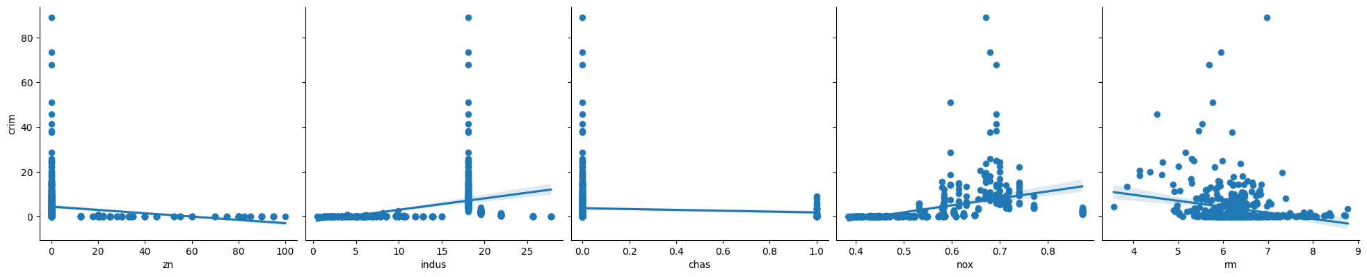
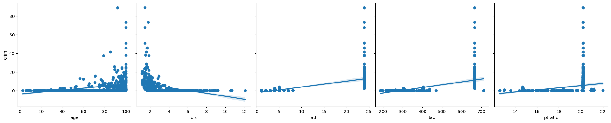
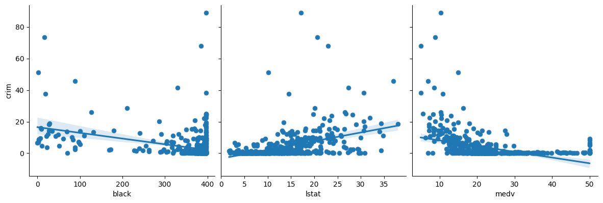
2. In which of the models is there a statistically significant association between the predictor and the response? Create some plots to back up your assertions.
# Write your code below to answer the question
Compare your answer with the reference solution below
print("p < 0.05\n")

for model in models_a:
    if model.pvalues[1] < 0.05:
        print(model.params[1:].index[0])

print("\np > 0.05\n")

for model in models_a:
    if model.pvalues[1] > 0.05:
        print(model.params[1:].index[0])

#  zn, indu,s nox, rm, ag, dis, rad, tax, ptratio, black, lstat, medv  are higly significant with very small p values.


def plot_grid(df, response, cols):
    variables = df.columns.drop(response)
    for i in range(0, len(variables), cols):
        g = sns.pairplot(
            df, y_vars=[response], x_vars=variables[i : i + cols], height=4
        )
        g.map(sns.regplot)
    return


plot_grid(boston_df, "crim", 5)
p < 0.05

zn
indus
nox
rm
age
dis
rad
tax
ptratio
black
lstat
medv

p > 0.05

chas
3. Fit a multiple regression model to predict the response using all of the predictors. Hint: See section 2.3.3.
# Write your code below to answer the question
Compare your answer with the reference solution below
response = "crim"
predictors = boston_df.columns.drop(response)
f = "{} ~ {}".format(response, "+".join(predictors))

model_b = ols(formula=f, data=boston_df).fit()
model_b.summary()
| Dep. Variable: | crim | R-squared: | 0.454 |
|---|---|---|---|
| Model: | OLS | Adj. R-squared: | 0.440 |
| Method: | Least Squares | F-statistic: | 31.47 |
| Date: | Tue, 06 Feb 2024 | Prob (F-statistic): | 1.57e-56 |
| Time: | 20:20:16 | Log-Likelihood: | -1653.3 |
| No. Observations: | 506 | AIC: | 3335. |
| Df Residuals: | 492 | BIC: | 3394. |
| Df Model: | 13 | ||
| Covariance Type: | nonrobust |
| coef | std err | t | P>|t| | [0.025 | 0.975] | |
|---|---|---|---|---|---|---|
| Intercept | 17.0332 | 7.235 | 2.354 | 0.019 | 2.818 | 31.248 |
| zn | 0.0449 | 0.019 | 2.394 | 0.017 | 0.008 | 0.082 |
| indus | -0.0639 | 0.083 | -0.766 | 0.444 | -0.228 | 0.100 |
| chas | -0.7491 | 1.180 | -0.635 | 0.526 | -3.068 | 1.570 |
| nox | -10.3135 | 5.276 | -1.955 | 0.051 | -20.679 | 0.052 |
| rm | 0.4301 | 0.613 | 0.702 | 0.483 | -0.774 | 1.634 |
| age | 0.0015 | 0.018 | 0.081 | 0.935 | -0.034 | 0.037 |
| dis | -0.9872 | 0.282 | -3.503 | 0.001 | -1.541 | -0.433 |
| rad | 0.5882 | 0.088 | 6.680 | 0.000 | 0.415 | 0.761 |
| tax | -0.0038 | 0.005 | -0.733 | 0.464 | -0.014 | 0.006 |
| ptratio | -0.2711 | 0.186 | -1.454 | 0.147 | -0.637 | 0.095 |
| black | -0.0075 | 0.004 | -2.052 | 0.041 | -0.015 | -0.000 |
| lstat | 0.1262 | 0.076 | 1.667 | 0.096 | -0.023 | 0.275 |
| medv | -0.1989 | 0.061 | -3.287 | 0.001 | -0.318 | -0.080 |
| Omnibus: | 666.613 | Durbin-Watson: | 1.519 |
|---|---|---|---|
| Prob(Omnibus): | 0.000 | Jarque-Bera (JB): | 84887.625 |
| Skew: | 6.617 | Prob(JB): | 0.00 |
| Kurtosis: | 65.058 | Cond. No. | 1.58e+04 |
Notes:
[1] Standard Errors assume that the covariance matrix of the errors is correctly specified.
[2] The condition number is large, 1.58e+04. This might indicate that there are
strong multicollinearity or other numerical problems.
4. Which features seem to be statistically significant in this model?
# Write your code below to answer the question
Compare your answer with the reference solution below
print("p < 0.05\n")
model_b.pvalues[model_b.pvalues < 0.05]

# Only the resultent features seem to be statistically significant in this model.
p < 0.05
Intercept    1.894909e-02
zn           1.702489e-02
dis          5.022039e-04
rad          6.460451e-11
black        4.070233e-02
medv         1.086810e-03
dtype: float64
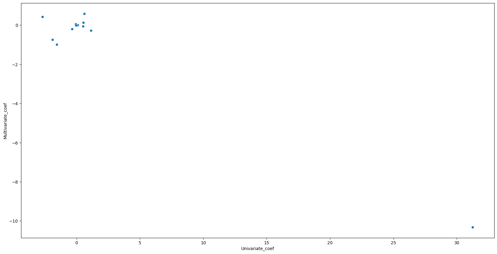
5. How do your results from Exercise 1 compare to your results from Exercise 3? Create a plot displaying the univariate regression coefficients from Exercise 1 on the \(x\)-axis, and the multiple regression coefficients from Exercise 3 on the \(y\)-axis. That is, each predictor is displayed as a single point in the plot. Its coefficient in a simple linear regression model is shown on the \(x\)-axis, and its coefficient estimate in the multiple linear regression model is shown on the \(y\)-axis.
# Write your code below to answer the question
Compare your answer with the reference solution below
# Get coefficients
univariate_params = pd.concat([m.params[1:] for m in models_a])
multivariate_params = model_b.params[1:]
df = pd.DataFrame(
    {
        "Univariate_coef": univariate_params,
        "Multivariate_coef": multivariate_params,
    }
)
print(df)

plt.figure(figsize=(20, 10))
ax = sns.scatterplot(x="Univariate_coef", y="Multivariate_coef", data=df)

# Multivariate regression found 5 of 13 predictors to be significnat where univariate regression found 12 of 13 significant. Multivariate regression seems to find significanlty less predictors to be significant.
         Univariate_coef  Multivariate_coef
zn             -0.073935           0.044855
indus           0.509776          -0.063855
chas           -1.892777          -0.749134
nox            31.248531         -10.313535
rm             -2.684051           0.430131
age             0.107786           0.001452
dis            -1.550902          -0.987176
rad             0.617911           0.588209
tax             0.029742          -0.003780
ptratio         1.151983          -0.271081
black          -0.036280          -0.007538
lstat           0.548805           0.126211
medv           -0.363160          -0.198887
6. Is there evidence of nonlinear association between any of the predictors and the response? To answer this question, for each predictor \(X\), fit a model of the form
Hint: See section 2.3.3.2.
# Write your code below to answer the question
Compare your answer with the reference solution below
models_d = [
    ols(
        formula="crim ~ {0} + np.power({0}, 2) + np.power({0}, 3)".format(f),
        data=boston_df,
    ).fit()
    for f in boston_df.columns[1:]
]

for model in models_d:
    print(model.summary().tables[1])


print("\nFeatures with p < 0.05\n")

sig = pd.concat([model.pvalues[model.pvalues < 0.05] for model in models_d])

print(pd.DataFrame({"P>|t|": sig.drop("Intercept")}))

# There is evidence of a nonlinear association between the repsonse and INDUS, NOX, AGE, DIS, PTRATIO, medv
# There is evidence of a linear association between the response and ZN
===================================================================================
                      coef    std err          t      P>|t|      [0.025      0.975]
-----------------------------------------------------------------------------------
Intercept           4.8461      0.433     11.192      0.000       3.995       5.697
zn                 -0.3322      0.110     -3.025      0.003      -0.548      -0.116
np.power(zn, 2)     0.0065      0.004      1.679      0.094      -0.001       0.014
np.power(zn, 3) -3.776e-05   3.14e-05     -1.203      0.230   -9.94e-05    2.39e-05
===================================================================================
======================================================================================
                         coef    std err          t      P>|t|      [0.025      0.975]
--------------------------------------------------------------------------------------
Intercept              3.6626      1.574      2.327      0.020       0.570       6.755
indus                 -1.9652      0.482     -4.077      0.000      -2.912      -1.018
np.power(indus, 2)     0.2519      0.039      6.407      0.000       0.175       0.329
np.power(indus, 3)    -0.0070      0.001     -7.292      0.000      -0.009      -0.005
======================================================================================
=====================================================================================
                        coef    std err          t      P>|t|      [0.025      0.975]
-------------------------------------------------------------------------------------
Intercept             3.7444      0.396      9.453      0.000       2.966       4.523
chas                 -0.6309      0.502     -1.257      0.209      -1.617       0.355
np.power(chas, 2)    -0.6309      0.502     -1.257      0.209      -1.617       0.355
np.power(chas, 3)    -0.6309      0.502     -1.257      0.209      -1.617       0.355
=====================================================================================
====================================================================================
                       coef    std err          t      P>|t|      [0.025      0.975]
------------------------------------------------------------------------------------
Intercept          233.0866     33.643      6.928      0.000     166.988     299.185
nox              -1279.3713    170.397     -7.508      0.000   -1614.151    -944.591
np.power(nox, 2)  2248.5441    279.899      8.033      0.000    1698.626    2798.462
np.power(nox, 3) -1245.7029    149.282     -8.345      0.000   -1538.997    -952.409
====================================================================================
===================================================================================
                      coef    std err          t      P>|t|      [0.025      0.975]
-----------------------------------------------------------------------------------
Intercept         112.6246     64.517      1.746      0.081     -14.132     239.382
rm                -39.1501     31.311     -1.250      0.212    -100.668      22.368
np.power(rm, 2)     4.5509      5.010      0.908      0.364      -5.292      14.394
np.power(rm, 3)    -0.1745      0.264     -0.662      0.509      -0.693       0.344
===================================================================================
====================================================================================
                       coef    std err          t      P>|t|      [0.025      0.975]
------------------------------------------------------------------------------------
Intercept           -2.5488      2.769     -0.920      0.358      -7.989       2.892
age                  0.2737      0.186      1.468      0.143      -0.093       0.640
np.power(age, 2)    -0.0072      0.004     -1.988      0.047      -0.014    -8.4e-05
np.power(age, 3)  5.745e-05   2.11e-05      2.724      0.007     1.6e-05    9.89e-05
====================================================================================
====================================================================================
                       coef    std err          t      P>|t|      [0.025      0.975]
------------------------------------------------------------------------------------
Intercept           30.0476      2.446     12.285      0.000      25.242      34.853
dis                -15.5544      1.736     -8.960      0.000     -18.965     -12.144
np.power(dis, 2)     2.4521      0.346      7.078      0.000       1.771       3.133
np.power(dis, 3)    -0.1186      0.020     -5.814      0.000      -0.159      -0.079
====================================================================================
====================================================================================
                       coef    std err          t      P>|t|      [0.025      0.975]
------------------------------------------------------------------------------------
Intercept           -0.6055      2.050     -0.295      0.768      -4.633       3.422
rad                  0.5127      1.044      0.491      0.623      -1.538       2.563
np.power(rad, 2)    -0.0752      0.149     -0.506      0.613      -0.367       0.217
np.power(rad, 3)     0.0032      0.005      0.703      0.482      -0.006       0.012
====================================================================================
====================================================================================
                       coef    std err          t      P>|t|      [0.025      0.975]
------------------------------------------------------------------------------------
Intercept           19.1836     11.796      1.626      0.105      -3.991      42.358
tax                 -0.1533      0.096     -1.602      0.110      -0.341       0.035
np.power(tax, 2)     0.0004      0.000      1.488      0.137      -0.000       0.001
np.power(tax, 3) -2.204e-07   1.89e-07     -1.167      0.244   -5.91e-07    1.51e-07
====================================================================================
========================================================================================
                           coef    std err          t      P>|t|      [0.025      0.975]
----------------------------------------------------------------------------------------
Intercept              477.1840    156.795      3.043      0.002     169.129     785.239
ptratio                -82.3605     27.644     -2.979      0.003    -136.673     -28.048
np.power(ptratio, 2)     4.6353      1.608      2.882      0.004       1.475       7.795
np.power(ptratio, 3)    -0.0848      0.031     -2.743      0.006      -0.145      -0.024
========================================================================================
======================================================================================
                         coef    std err          t      P>|t|      [0.025      0.975]
--------------------------------------------------------------------------------------
Intercept             18.2637      2.305      7.924      0.000      13.735      22.792
black                 -0.0836      0.056     -1.483      0.139      -0.194       0.027
np.power(black, 2)     0.0002      0.000      0.716      0.474      -0.000       0.001
np.power(black, 3) -2.652e-07   4.36e-07     -0.608      0.544   -1.12e-06    5.92e-07
======================================================================================
======================================================================================
                         coef    std err          t      P>|t|      [0.025      0.975]
--------------------------------------------------------------------------------------
Intercept              1.2010      2.029      0.592      0.554      -2.785       5.187
lstat                 -0.4491      0.465     -0.966      0.335      -1.362       0.464
np.power(lstat, 2)     0.0558      0.030      1.852      0.065      -0.003       0.115
np.power(lstat, 3)    -0.0009      0.001     -1.517      0.130      -0.002       0.000
======================================================================================
=====================================================================================
                        coef    std err          t      P>|t|      [0.025      0.975]
-------------------------------------------------------------------------------------
Intercept            53.1655      3.356     15.840      0.000      46.571      59.760
medv                 -5.0948      0.434    -11.744      0.000      -5.947      -4.242
np.power(medv, 2)     0.1555      0.017      9.046      0.000       0.122       0.189
np.power(medv, 3)    -0.0015      0.000     -7.312      0.000      -0.002      -0.001
=====================================================================================

Features with p < 0.05

                             P>|t|
zn                    2.612296e-03
indus                 5.297064e-05
np.power(indus, 2)    3.420187e-10
np.power(indus, 3)    1.196405e-12
nox                   2.758372e-13
np.power(nox, 2)      6.811300e-15
np.power(nox, 3)      6.961110e-16
np.power(age, 2)      4.737733e-02
np.power(age, 3)      6.679915e-03
dis                   6.374792e-18
np.power(dis, 2)      4.941214e-12
np.power(dis, 3)      1.088832e-08
ptratio               3.028663e-03
np.power(ptratio, 2)  4.119552e-03
np.power(ptratio, 3)  6.300514e-03
medv                  2.637707e-28
np.power(medv, 2)     3.260523e-18
np.power(medv, 3)     1.046510e-12
7. Compare the differences between a linear regression model and a quadratic regression model for regressing ptratio onto crim. Does the quadratic term improves the fit to the data? Hint: See section 2.3.3.3.
# Write your code below to answer the question
Compare your answer with the reference solution below
from sklearn.linear_model import LinearRegression
import matplotlib.pyplot as plt
import seaborn as sns

regr = LinearRegression()

# Linear fit
X = boston_df.ptratio.values.reshape(-1, 1)
y = boston_df.crim
regr.fit(X, y)

boston_df["pred1"] = regr.predict(X)
boston_df["resid1"] = boston_df.crim - boston_df.pred1


boston_df["ptratio2"] = boston_df.ptratio**2
# Quadratic fit
X2 = boston_df[["ptratio", "ptratio2"]].values
regr.fit(X2, y)

boston_df["pred2"] = regr.predict(X2)
boston_df["resid2"] = boston_df.crim - boston_df.pred2


fig, (ax1, ax2) = plt.subplots(1, 2, figsize=(12, 5))

# Left plot
sns.regplot(
    x=boston_df.pred1,
    y=boston_df.resid1,
    lowess=True,
    ax=ax1,
    line_kws={"color": "r", "lw": 1},
    scatter_kws={"facecolors": "None", "edgecolors": "k", "alpha": 0.5},
)
ax1.hlines(
    0,
    xmin=ax1.xaxis.get_data_interval()[0],
    xmax=ax1.xaxis.get_data_interval()[1],
    linestyles="dotted",
)
ax1.set_title("Residual Plot for Linear Fit")

# Right plot
sns.regplot(
    x=boston_df.pred2,
    y=boston_df.resid2,
    lowess=True,
    line_kws={"color": "r", "lw": 1},
    ax=ax2,
    scatter_kws={"facecolors": "None", "edgecolors": "k", "alpha": 0.5},
)
ax2.hlines(
    0,
    xmin=ax2.xaxis.get_data_interval()[0],
    xmax=ax2.xaxis.get_data_interval()[1],
    linestyles="dotted",
)
ax2.set_title("Residual Plot for Quadratic Fit")

for ax in fig.axes:
    ax.set_xlabel("Fitted values")
    ax.set_ylabel("Residuals")

# The left plot displays a residual plot from the linear regression of ptratio onto crim on the Boston dataset.
# The red line is a smooth fit to the residuals for identifying any trends in the residuals.
# Here, the residuals exhibit a tendency of U-shape, which provides a strong indication of nonlinearity in the data.


# The right panel displays the residual plot that results from the model contains a quadratic term.
# There appears to be little pattern in the residuals, suggesting that the quadratic term improves the fit to the data.