Multiple linear regression
Contents
2.2. Multiple linear regression
Read then Launch
This content is best viewed in html because jupyter notebook cannot display some content (e.g. figures, equations) properly. You should finish reading this page first and then launch it as an interactive notebook in Google Colab (faster, Google account needed) or Binder by clicking the rocket symbol () at the top.
We have examined the relationship between sale and TV of the Advertising dataset for simple linear regression. There are two more predictor variables radio and newspaper in the dataset. How can we account for the effect of these two variables in the model?
Watch the 5-minute video below for a visual explanation of multiple linear regression.
Video
Explaining Multiple Linear Regression by StatQuest, embedded according to YouTube’s Terms of Service.
Then study the following sections to learn more about multiple linear regression with examples in the textbook.
2.2.1. Install libraries
If you are using Google Colab, please uncomment the following code to update the version of matplotlib. Once complete, click the RESTART RUNTIME button to restart the runtime in order to use newly installed versions.
# !pip install -q mpl_toolkits statsmodels
2.2.2. Import libraries and load data
Get ready by importing the APIs needed from respective libraries.
# %load ../standard_import.txt
import pandas as pd
import numpy as np
import matplotlib.pyplot as plt
from mpl_toolkits.mplot3d import axes3d

from sklearn.linear_model import LinearRegression
from statsmodels.formula.api import ols

%matplotlib inline
Load Datasets
Load the Advertising dataset.
data_url = "https://github.com/pykale/transparentML/raw/main/data/Advertising.csv"
advertising_df = pd.read_csv(data_url, header=0, index_col=0)
To accommodate multiple predictor variables, one option is to run simple linear regression separately for each predictor variable.
The following code runs a simple linear regression model of radio, and newspaper onto sales using statsmodels, respectively (Table 3.3 in the textbook).
est = ols("Sales ~ Radio", advertising_df).fit()
est.summary().tables[1]
| coef | std err | t | P>|t| | [0.025 | 0.975] | |
|---|---|---|---|---|---|---|
| Intercept | 9.3116 | 0.563 | 16.542 | 0.000 | 8.202 | 10.422 |
| Radio | 0.2025 | 0.020 | 9.921 | 0.000 | 0.162 | 0.243 |
est = ols("Sales ~ Newspaper", advertising_df).fit()
est.summary().tables[1]
| coef | std err | t | P>|t| | [0.025 | 0.975] | |
|---|---|---|---|---|---|---|
| Intercept | 12.3514 | 0.621 | 19.876 | 0.000 | 11.126 | 13.577 |
| Newspaper | 0.0547 | 0.017 | 3.300 | 0.001 | 0.022 | 0.087 |
However, fitting a separate simple linear regression model for each predictor is problematic: 1) It is unclear how to make a single prediction given the three advertising media budgets; 2) each separate linear regression model ignores the effect of the other two predictors, which can lead to misleading estimates.
A better approach is to use multiple linear regression. Multiple linear regression is an extension of simple linear regression. It allows us to predict a quantitative response using more than one predictor variable. The equation for a multiple linear regression model with \(D\) predictor variables is given by:
where \(y\) is the response, \(x_1, x_2, ..., x_D\) are the \(D\) predictors, \(D\) is the total number of predictor variables (features), and \(\epsilon\) is the error term. The \(\beta\)s are called the regression coefficients, where \(\beta_0\) is the bias (intercept), and \(\beta_1, \beta_2, ..., \beta_D\) are the weights (slopes). Considering \(N\) samples, the equation can be written in matrix form as:
where \(\mathbf{y}\) is an \(N \times 1\) vector of responses, \(\mathbf{X}\) is an \(N \times (D+1)\) matrix of predictors, \(\boldsymbol{\beta}\) is a \((D+1) \times 1\) vector of regression coefficients, and \(\boldsymbol{\epsilon}\) is an \(N \times 1\) vector of errors. The predictor (feature) matrix \(\mathbf{X}\) contains a column of 1s to account for the intercept. The vector \(\boldsymbol{\beta}\) contains the intercept in the first position and the slopes for the remaining \(D\) predictors. The vector \(\boldsymbol{\epsilon}\) contains the error terms for each observation.
Using the Advertising dataset as an example, we can fit a multiple linear regression model to the three predictor variables TV, radio, and newspaper to predict sales as follows:
2.2.3. Estimating the regression coefficients
Similar to simple linear regression, we can estimate the regression coefficients using least squares. The least squares estimates for the regression coefficients are given by:
where \(y_i\) is the \(i\)th response, \(\hat{y}_i\) is the \(i\)th predicted response, \(\hat{\beta}_0\) is the intercept, \(\hat{\beta}_1\) is the slope for \(x_{i1}\), \(\hat{\beta}_2\) is the slope for \(x_{i2}\), and so on. \(\hat{\beta}\)s are the least squares estimates for the regression coefficients, which can be obtained in matrix form as:
The following code run a multiple linear regression model to regress TV, radio, and newspaper onto sales using statsmodels, and display the learnt coefficients (Table 3.4 in the textbook).
est = ols("Sales ~ TV + Radio + Newspaper", advertising_df).fit()
est.summary()
| Dep. Variable: | Sales | R-squared: | 0.897 |
|---|---|---|---|
| Model: | OLS | Adj. R-squared: | 0.896 |
| Method: | Least Squares | F-statistic: | 570.3 |
| Date: | Tue, 06 Feb 2024 | Prob (F-statistic): | 1.58e-96 |
| Time: | 20:20:20 | Log-Likelihood: | -386.18 |
| No. Observations: | 200 | AIC: | 780.4 |
| Df Residuals: | 196 | BIC: | 793.6 |
| Df Model: | 3 | ||
| Covariance Type: | nonrobust |
| coef | std err | t | P>|t| | [0.025 | 0.975] | |
|---|---|---|---|---|---|---|
| Intercept | 2.9389 | 0.312 | 9.422 | 0.000 | 2.324 | 3.554 |
| TV | 0.0458 | 0.001 | 32.809 | 0.000 | 0.043 | 0.049 |
| Radio | 0.1885 | 0.009 | 21.893 | 0.000 | 0.172 | 0.206 |
| Newspaper | -0.0010 | 0.006 | -0.177 | 0.860 | -0.013 | 0.011 |
| Omnibus: | 60.414 | Durbin-Watson: | 2.084 |
|---|---|---|---|
| Prob(Omnibus): | 0.000 | Jarque-Bera (JB): | 151.241 |
| Skew: | -1.327 | Prob(JB): | 1.44e-33 |
| Kurtosis: | 6.332 | Cond. No. | 454. |
Notes:
[1] Standard Errors assume that the covariance matrix of the errors is correctly specified.
2.2.4. Interpreting the results
We have interpreted the results of simple linear regression in the previous section. The interpretation of the results of multiple linear regression is similar. The only difference is that there are now three coefficients to interpret.
Challenge
Interpret the results of the multiple linear regression model above based on the previous section and then click the following to compare the provided interpretation with yours.
How to interpret the results?
We interpret these results above as follows:
For a given (i.e. fixed) amount of
TVandnewspaperadvertising budgets, spending an additional $1,000 onradioadvertising is associated with approximately 189 units of additionalsales(recall the units of the variables).Comparing these coefficients to the estimates in simple linear regression, we notice that the multiple regression coefficient estimates for
TVandradioare pretty similar to the simple linear regression coefficient estimates. However, while thenewspaperregression coefficient estimate in simple linear regression was significantly non-zero, the coefficient estimate fornewspaperin the multiple regression model is close to zero, and the corresponding \(p\)-value is no longer significant, with a value around 0.86.This illustrates that the simple and multiple regression coefficients can be quite different. This difference stems from the fact that in the simple regression case, the slope term represents the average increase in product sales associated with a $1,000 increase in newspaper advertising, ignoring other predictors such as
TVandradio. By contrast, in the multiple regression setting, the coefficient fornewspaperrepresents the average increase in productsalesassociated with increasingnewspaperspending by $1,000 while holdingTVandradiofixed.
Why the relationship between sales and newspaper are opposite in the simple linear regression and multiple linear regression? Use following code displays the correlation matrix of the Advertising dataset for further analysis.
advertising_df.corr()
| TV | Radio | Newspaper | Sales | |
|---|---|---|---|---|
| TV | 1.000000 | 0.054809 | 0.056648 | 0.782224 |
| Radio | 0.054809 | 1.000000 | 0.354104 | 0.576223 |
| Newspaper | 0.056648 | 0.354104 | 1.000000 | 0.228299 |
| Sales | 0.782224 | 0.576223 | 0.228299 | 1.000000 |
How to interpret the results?
The correlation between radio and newspaper is 0.35, which is much higher than the other pair-wise correlations among the three medias. This indicates that in those markets spending more on newspaper (radio) advertising, there is a tendency to spend more on radio (newspaper) advertising as well.
Now suppose that the multiple regression is correct and newspaper advertising is not associated with sales, but radio advertising is associated with sales. Then in markets where we spend more on radio, our sales will tend to be higher. As our correlation matrix shows, we also tend to spend more on newspaper advertising in those same markets. Hence, in a simple linear regression which only examines sales versus newspaper, we will observe that higher values of newspaper tend to be associated with higher values of sales, even though newspaper advertising is not directly associated with sales. So newspaper advertising is a surrogate for radio advertising; newspaper gets “credit” for the association between radio on sales.
2.2.5. Important questions in multiple linear regression
2.2.5.1. Is at least one of the predictors \(x_1, x_2, ..., x_D\) useful in predicting the response?
We can answer this question by testing the null hypothesis that all the regression coefficients are zero, i.e.
versus the alternative hypothesis that at least one of the regression coefficients is non-zero, i.e.:
This hypothesis test is performed by computing the \(F\)-statistic, which is defined as:
where \(\text{TSS} = \sum(y_i - \bar{y})^2\) and \(\text{RSS} = \sum(y_i - \hat{y}_i)^2\). Remember, \(y_i\) is the \(i\)th target, \(\hat{y}_i\) is the \(i\)th prediction and \(\bar{y}\) is the sample mean. When there is no relationship between the response and predictors, one would expect the \(F\)-statistic to take on a value close to 1. On the other hand, if \(H_1\) a is true, we can expect \(F\) to be greater than 1.
The \(F\)-statistic for the multiple linear regression model obtained by regressing sales onto radio, TV, and newspaper is 570.3 (displayed in the first regression results in a previous section). Since this is far greater than 1, it provides compelling evidence against the null hypothesis \(H_0\). In other words, the large \(F\)-statistic suggests that at least one of the advertising media must be related to sales.
Watch the following 9-minute video excerpt to learn more about the \(F\)-statistic.
Video
Calculating a \(p\)-value for \(R^2\) by StatQuest, embedded according to YouTube’s Terms of Service.
2.2.5.2. Do all the predictors help to explain \(y\), or is only a subset of the predictors useful?
It is possible that the response is only associated with a subset of the predictors. The task of determining which subset of predictors are (most) associated with the response is referred to as variable selection (or feature selection). This will be discussed in more detail in Feature Selection and Regularisation.
There are three common approaches to variable selection:
Forward selection. We begin with a model containing no predictors, and then consider adding predictors one at a time until all predictors have been considered. The best single predictor is added to the model, and the process is repeated until all predictors have been added to the model. This is a greedy algorithm, and it is not guaranteed to find the best model containing a subset of the predictors.
Backward selection. We begin with a model containing all predictors, and then consider removing predictors one at a time until no predictors remain. The worst single predictor is removed from the model, and the process is repeated until no predictors remain in the model. This is also a greedy algorithm, and it is not guaranteed to find the best model containing a subset of the predictors.
Mixed selection. We begin with some initial model containing a subset of the predictors. We then consider adding or removing each predictor individually, and retain the best model that results. This is also a greedy algorithm, and it is not guaranteed to find the best model containing a subset of the predictors.
2.2.5.3. How well does the model fit the data?
Similar to simple linear regression. We can answer this question by computing the \(R^2\) and RSE statistics. The \(R^2\) for multiple linear regression is defined in the same way as in simple linear regression as:
The \(R^2\) statistic provides an indication of the proportion of the variance in the response that is predictable from the predictors. In this case, the \(R^2\) statistic is 0.897, which indicates that 89.7% of the variance in sales is predictable from TV, radio, and newspaper.
The RSE for multiple linear regression is defined as:
You can verify that when \(D=1\), the RSE for multiple linear regression is the same as the RSE for simple linear regression.
Run the following code to fit and then evaluate a multiple linear regression model using scikit-learn:
Firstly, fit a linear regression to sales using TV and radio as predictors.
regr = LinearRegression()

X = advertising_df[["Radio", "TV"]].values
y = advertising_df.Sales

regr.fit(X, y)
print(regr.coef_)
print(regr.intercept_)
[0.18799423 0.04575482]
2.9210999124051398
Find out the min/max values of Radio & TV to set up the grid (range) for plotting.
advertising_df[["Radio", "TV"]].describe()
| Radio | TV | |
|---|---|---|
| count | 200.000000 | 200.000000 |
| mean | 23.264000 | 147.042500 |
| std | 14.846809 | 85.854236 |
| min | 0.000000 | 0.700000 |
| 25% | 9.975000 | 74.375000 |
| 50% | 22.900000 | 149.750000 |
| 75% | 36.525000 | 218.825000 |
| max | 49.600000 | 296.400000 |
Create a coordinate grid
radio = np.arange(0, 50)
tv = np.arange(0, 300)

beta_1, beta_2 = np.meshgrid(radio, tv, indexing="xy")
Z = np.zeros((tv.size, radio.size))

for (i, j), v in np.ndenumerate(Z):
    Z[i, j] = (
        regr.intercept_ + beta_1[i, j] * regr.coef_[0] + beta_2[i, j] * regr.coef_[1]
    )
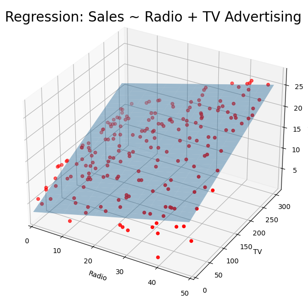
Create 3D plot of sales vs TV and radio.
# Create plot
fig = plt.figure(figsize=(10, 6))
fig.suptitle("Regression: Sales ~ Radio + TV Advertising", fontsize=20)

ax = axes3d.Axes3D(fig, auto_add_to_figure=False)
fig.add_axes(ax)

ax.plot_surface(beta_1, beta_2, Z, rstride=10, cstride=5, alpha=0.4)
ax.scatter3D(advertising_df.Radio, advertising_df.TV, advertising_df.Sales, c="r")

ax.set_xlabel("Radio")
ax.set_xlim(0, 50)
ax.set_ylabel("TV")
ax.set_ylim(bottom=0)
ax.set_zlabel("Sales")
plt.show()
2.2.5.4. Given a set of predictor values, what response value should we predict, and how accurate is our prediction?
Once we have fit a multiple linear regression model, we can use the model to make predictions of the response for a given set of predictor values.
However, we must be careful when making predictions, because the observed values of the predictors may not have been part of the data used to fit the model. In this case, the prediction may not be very accurate and using a confidence interval can help quantify the uncertainty associated with the prediction.
2.2.6. Exercise
1. All the following exercises involve the use of the Carseats dataset. Fit a multiple regression model to predict Sales using Price, Income, and CompPrice. Hint: See section 2.2.5.
# Write your code below to answer the question
Compare your answer with the reference solution below
import pandas as pd
import numpy as np
from sklearn.preprocessing import StandardScaler
from sklearn.linear_model import LinearRegression

# Load data
carseats_df = pd.read_csv(
    "https://github.com/pykale/transparentML/raw/main/data/Carseats.csv"
)

regr = LinearRegression()

X = carseats_df[["Price", "Income", "CompPrice"]].values
y = carseats_df.Sales

regr.fit(X, y)
print("Regression model slop/coeffcient (weight):", regr.coef_)
print("Regression model intercept (bias):", regr.intercept_)
Regression model slop/coeffcient (weight): [-0.08719674  0.01525145  0.09278583]
Regression model intercept (bias): 4.950235603666373
i. How well does the model fit the data?
# Write your code below to answer the question
Compare your answer with the reference solution below
from sklearn.metrics import mean_squared_error, r2_score

y_pred = regr.predict(X)
print("R2 score:", r2_score(y, y_pred))

# The model didn't fit the data well as the R2 score is still way below 1.
R2 score: 0.3805237817874102
ii. Does multiple linear regression help the model fit the data better than simpler linear regression (see simple linear regression exercises).
Compare your answer with the solution below
Yes. The \(R^2\) score has increased in multiple linear regression, and the MSE has decreased, which means the model performed better than simpler linear regression in terms of fitting the data.
iii. Write out the model in equation form.
Compare your answer with the solution below
\(\hat{y} = 4.95 + (-0.08719674 * Price) + (0.01525145 * Income) + (0.09278583 * CompPrice)\)
2. Find the correlation between Sales, Price, Income, and CompPrice and interpret the result. Hint: See section 2.2.4.
# Write your code below to answer the question
Compare your answer with the reference solution below
carseats_df[["Sales", "Price", "Income", "CompPrice"]].corr()

# The correlation between Price and CompPrice is 0.58, which is much higher than the other pair-wise correlations. This indicates that by increasing the component price(Price) of a caraseat, there is a tendency for the overall price(CompPrice) to increase as well.
| Sales | Price | Income | CompPrice | |
|---|---|---|---|---|
| Sales | 1.000000 | -0.444951 | 0.151951 | 0.064079 |
| Price | -0.444951 | 1.000000 | -0.056698 | 0.584848 |
| Income | 0.151951 | -0.056698 | 1.000000 | -0.080653 |
| CompPrice | 0.064079 | 0.584848 | -0.080653 | 1.000000 |
3. Perform a multiple linear regression using statsmodels library with Sales as the response and Price, Income, and CompPrice as predictors. Use the summary() function to print the results. Compare the regression coefficients/weights with Exercise 1. Hint: See section 2.2.3.
# Write your code below to answer the question
Compare your answer with the reference solution below
import patsy
import statsmodels.api as sm

f = "Sales ~ Price + Income + CompPrice"
y, X = patsy.dmatrices(f, carseats_df, return_type="dataframe")

model = sm.OLS(y, X).fit()
print(model.summary())

# The regression coeffcients are same as scikit learn model
                            OLS Regression Results
==============================================================================
Dep. Variable:                  Sales   R-squared:                       0.381
Model:                            OLS   Adj. R-squared:                  0.376
Method:                 Least Squares   F-statistic:                     81.08
Date:                Tue, 06 Feb 2024   Prob (F-statistic):           6.52e-41
Time:                        20:20:20   Log-Likelihood:                -886.58
No. Observations:                 400   AIC:                             1781.
Df Residuals:                     396   BIC:                             1797.
Df Model:                           3
Covariance Type:            nonrobust
==============================================================================
                 coef    std err          t      P>|t|      [0.025      0.975]
------------------------------------------------------------------------------
Intercept      4.9502      0.981      5.044      0.000       3.021       6.880
Price         -0.0872      0.006    -14.991      0.000      -0.099      -0.076
Income         0.0153      0.004      3.809      0.000       0.007       0.023
CompPrice      0.0928      0.009     10.315      0.000       0.075       0.110
==============================================================================
Omnibus:                        7.331   Durbin-Watson:                   1.884
Prob(Omnibus):                  0.026   Jarque-Bera (JB):                7.077
Skew:                           0.285   Prob(JB):                       0.0291
Kurtosis:                       2.683   Cond. No.                     1.63e+03
==============================================================================

Notes:
[1] Standard Errors assume that the covariance matrix of the errors is correctly specified.
[2] The condition number is large, 1.63e+03. This might indicate that there are
strong multicollinearity or other numerical problems.
4. From the model fitted in Exercise 3, for which predictors can you reject the null hypothesis \(H_0 : \beta_j = 0\) ? Hint: See section 2.2.5.
# Write your code below to answer the question
Compare your answer with the reference solution below
# The following predictors have p-values < 0.05 which suggests we can reject the null hypothesis
model.pvalues[model.pvalues < 0.05].sort_values()
Price        1.475505e-40
CompPrice    2.972755e-22
Intercept    6.951811e-07
Income       1.619686e-04
dtype: float64
i. Which predictors appear to have a statistically significant relationship with the response?
Compare your answer with the solution below
All predictors appear to have a statistically significant relationship to the response.
ii. What does the coefficient for the income variable suggest?
Compare your answer with the solution below
The coefficient for the income variable suggests that there is a positive relationship between income and sales, where the response variable increases as income increases.
5. Using the fitted model from Exercise 3, obtain \(95\%\) confidence intervals for the coefficients. Hint: See section 2.1.9.
# Write your code below to answer the question
Compare your answer with the reference solution below
# Extract 95% confidence intervals
conf_inter_95 = model.conf_int(alpha=0.05)
conf_inter_95.rename(
    index=str,
    columns={
        0: "min.",
        1: "max.",
    },
)
| min. | max. | |
|---|---|---|
| Intercept | 3.020863 | 6.879608 |
| Price | -0.098632 | -0.075762 |
| Income | 0.007379 | 0.023124 |
| CompPrice | 0.075101 | 0.110471 |