Regularisation
Contents
6.2. Regularisation
For the case of linear regression, the feature (subset) selection methods in the previous section involve using least squares to fit a linear model that contains a subset of the predictors (features/variables). We have seen the large variance of the least squares estimates across different folds in cross validation. This variance is related to the sensitivity of the least squares estimates to small changes in the data, leading to overfitting.
In this section, we will see how to reduce this variance by regularising the least squares estimates, i.e. regularisation. We can fit a model containing all \(D\) predictors using a technique that constrains or regularises the coefficient estimates, or equivalently, that shrinks the coefficient estimates towards zero and significantly reduce their variance. The two best-known techniques for shrinking the regression coefficients towards zero, i.e. regularisation, are ridge regression and the lasso.
6.2.1. Ridge regression
Recall from Linear regression that the least squares fitting procedure estimates \(\beta_0, \beta_1, \ldots, \beta_D\) by minimising the residual sum of squares (RSS) on the training data:
Ridge regression is very similar to least squares, except that the coefficients are estimated by minimizing a slightly different quantity. In particular, the ridge regression coefficient estimates \(\beta^R\) are the values that minimise
where \(\lambda \geq 0\) is a tuning (or regularisation) parameter. The term \(\lambda \sum_{d=1}^D \beta_d^2\) is called a regularisation term (or shrinkage penalty), because it regularises (shrinks) the coefficient estimates towards zero. The tuning parameter \(\lambda\) controls the amount of shrinkage: for large values of \(\lambda\), the coefficients are very strongly shrunk towards zero, whereas for small values of \(\lambda\), the coefficients are barely shrunk at all. In the limit as \(\lambda \rightarrow 0\), ridge regression recovers the least squares estimates, i.e. degenerated to linear regression without regularisation.
Note that the regularisation term in ridge regression has the effect of shrinking the coefficient estimates \(\beta_d\) for all \(d\), but it has no effect on \(\beta_0\). This is because the penalty only includes the sum of squares of the \(\beta_d\), not the \(\beta_0\). In other words, the penalty has no effect on the intercept. This is a desirable property, since we usually do not want to regularise the intercept.
Watch the 9-minute video below for a visual explanation of ridge regression:
Video
Explaining Ridge regression by StatQuest, embedded according to YouTube’s Terms of Service.
6.2.1.1. Ridge regression on Credit dataset
Let us perform a ridge regression on the Credit dataset to predict the Balance using all the other variables. We will use the scikit-learn implementation of ridge regression, which can be found in the sklearn.linear_model.Ridge class. The alpha parameter is our \(lambda\) that controls the amount of regularisation (shrinkage): the larger the value of alpha, the greater the amount of shrinkage.
Get ready by importing the APIs needed from respective libraries.
import matplotlib.pyplot as plt
import numpy as np
import pandas as pd
from sklearn.linear_model import Ridge, Lasso
from sklearn.metrics import mean_squared_error
from sklearn.model_selection import train_test_split
from sklearn.preprocessing import StandardScaler

%matplotlib inline
Set a random seed for reproducibility.
np.random.seed(2022)
Load the Credit dataset dataset, convert the values of variables (predictors) Student, Own, Married, and Region from category to numbers (‘0’ and ‘1’), and inspect the first three rows.
credit_url = "https://github.com/pykale/transparentML/raw/main/data/Credit.csv"

credit_df = pd.read_csv(credit_url)
credit_df["Student2"] = credit_df.Student.map({"No": 0, "Yes": 1})
credit_df["Own2"] = credit_df.Own.map({"No": 0, "Yes": 1})
credit_df["Married2"] = credit_df.Married.map({"No": 0, "Yes": 1})
credit_df["South"] = credit_df.Region.map(
    {"South": 1, "North": 0, "West": 0, "East": 0}
)
credit_df["West"] = credit_df.Region.map({"West": 1, "North": 0, "South": 0, "East": 0})
credit_df["East"] = credit_df.Region.map({"East": 1, "North": 0, "South": 0, "West": 0})
# credit_df["Region2"] = credit_df.Region.astype("category")
credit_df.head(3)
| Income | Limit | Rating | Cards | Age | Education | Own | Student | Married | Region | Balance | Student2 | Own2 | Married2 | South | West | East | |
|---|---|---|---|---|---|---|---|---|---|---|---|---|---|---|---|---|---|
| 0 | 14.891 | 3606 | 283 | 2 | 34 | 11 | No | No | Yes | South | 333 | 0 | 0 | 1 | 1 | 0 | 0 |
| 1 | 106.025 | 6645 | 483 | 3 | 82 | 15 | Yes | Yes | Yes | West | 903 | 1 | 1 | 1 | 0 | 1 | 0 |
| 2 | 104.593 | 7075 | 514 | 4 | 71 | 11 | No | No | No | West | 580 | 0 | 0 | 0 | 0 | 1 | 0 |
Drop categorical variables, which have been converted to numerical variables, and the Balance variable, which is the target variable. Standardise the remaining variables.
X = credit_df.drop(["Own", "Student", "Married", "Region", "Balance"], axis=1).values
scaler = StandardScaler()
X_scaled = scaler.fit_transform(X)
y = credit_df.Balance.values
Choose a set of lambda values to study for ridge regression, using the np.logspace function. This function returns a set of values that are logarithmically spaced between the two specified values, which is useful for exploring a wide range of values at a small cost.
lambdas = np.logspace(-2, 4, 20)
coef_ridge = []

for lambda_ in lambdas:
    ridge = Ridge(alpha=lambda_)
    ridge.fit(X_scaled, y)
    coef_ridge.append(ridge.coef_)

coef_ridge = np.array(coef_ridge)
Plot the coefficient estimates for each of the lambda values.
plt.plot(lambdas, coef_ridge[:, 0], c="black", ls="-", label="Income")
plt.plot(lambdas, coef_ridge[:, 1], c="tab:red", ls="--", label="Limit")
plt.plot(lambdas, coef_ridge[:, 2], c="tab:blue", ls=":", label="Rating")
plt.plot(lambdas, coef_ridge[:, 6], c="orange", ls=":", label="Student")

plt.legend()
plt.xscale("log")
plt.ylim(-300, 500)
plt.xlabel(r"$\lambda$")
plt.ylabel("Standardised Coefficients")
plt.grid(True)
plt.show()
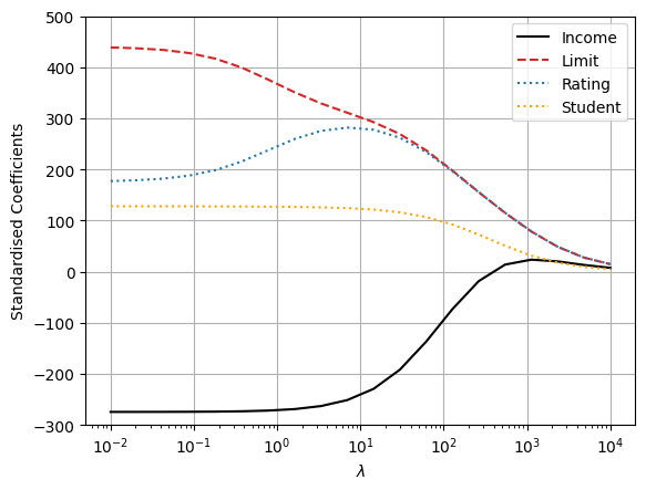
We can observe that the coefficient estimates approach zero as the value of lambda increases. This is because the regularisation term in ridge regression has the effect of shrinking the coefficient estimates towards zero. The coefficient estimates for lambda values close to zero are very similar to the least squares estimates, whereas the coefficient estimates for lambda values close to 10000 are very close to zero.
6.2.1.2. Bias–variance trade-off in ridge regression
So, why can ridge regression improve over least squares? Let us plot the mean squared error (MSE) on the test data for each of the lambda values, up to 100. We will use the sklearn.metrics.mean_squared_error function to compute the MSE.
label_scaler = StandardScaler()
X_train, X_test, y_train, y_test = train_test_split(
    X_scaled, y, test_size=0.1, random_state=123, shuffle=True
)
# Define Algorithm

mses = []

lambdas = np.logspace(-2, 2, 20)

for lambda_ in lambdas:
    ridge = Ridge(alpha=lambda_)
    ridge.fit(X_train, y_train)
    mses.append(mean_squared_error(y_test, ridge.predict(X_test)))

print("Best MSE: ", np.min(mses))

fig, ax = plt.subplots(figsize=(10, 6))

ax.plot(lambdas, mses, c="m", ls="-", label="$MSE(x)$")
ax.vlines(1, np.min(mses), np.max(mses), colors="k", ls="--", label="Optimal $\lambda$")

# add annotation
ax.annotate("Overfit (high variance, high bias)", xy=(0.01, 17000), fontsize=14)
ax.annotate(
    "",
    xy=(0.05, 14000),
    xytext=(0.05, 17000),
    arrowprops=dict(arrowstyle="->", relpos=(0, 0)),
)
ax.annotate(
    "Underfit (high bias, low variance)",
    xy=(70, 20000),
    xytext=(2, 23000),
    arrowprops=dict(arrowstyle="->"),
    fontsize=14,
)
ax.annotate("Optimal", xy=(5, 15000), fontsize=14)
ax.annotate(
    "",
    xy=(lambdas[np.argmin(mses)], np.min(mses)),
    xytext=(lambdas[np.argmin(mses)], 15000),
    arrowprops=dict(arrowstyle="->", relpos=(0, 0)),
)

plt.xscale("log")
plt.yscale("log")
plt.xlabel(r"$\lambda$")
plt.ylabel("Mean Squared Error")
plt.grid(True)
plt.show()
Best MSE: 12385.885432230525
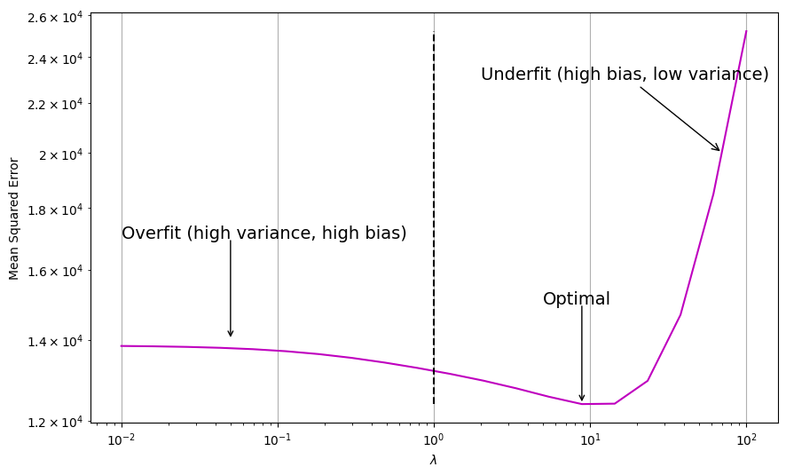
Ridge regression’s advantage over least squares is that it can alleviate overfitting, which is rooted in the bias-variance trade-off. As \(\lambda\) increases, the flexibility of the ridge regression fit decreases, leading to decreased variance but increased bias. In other words, ridge regression reduces the variance of the least squares estimates, but at the expense of increasing the bias. As shown in the figure above, for values of \(\lambda\) up to about 10, the MSE drops as \(\lambda\) increases. Beyond this point, the MSE increases considerably. This is because the bias introduced by ridge regression becomes too large, and the model becomes too rigid to to capture the true relationship between the predictors and the response.
Bias-variance trade-off
Variance refers to the amount by which \(\hat{f}(\mathbf{x})\) would change if we estimated it using a different training dataset. If a method has high variance, then small changes in the training data can result in large changes in the estimated values of \(\hat{f}(\mathbf{x})\).
Bias refers to the error that is introduced by approximating a real-life problem, which may be extremely complicated, by a much simpler model. For example, linear regression assumes a linear relationship between the predictors and the response, but many real-life relationships are nonlinear. In this case, the linear regression model will have high bias, since it will not be able to capture the nonlinear relationship between the predictors and the response.
Generally, more flexible methods have higher variance and lower bias, and less flexible methods (such as linear methods) have lower variance and higher bias.
To better understand this trade-off, let us consider the mean square error (MSE), which can be decomposed into multiple components as:
where \(\mathbb{E}[\cdot]\) is the expectation operator. The first term on the right-hand side is the squared bias, the second term is the variance of the prediction, and the third term is the irreducible error.
The bias-variance trade-off is a consequence of the fact that the variance and squared bias terms are inversely related. As the variance increases, the squared bias decreases, and vice versa. The irreducible error is the variance of the error term \(\epsilon\) and is independent of the model. The MSE is minimised when the variance and squared bias are equal, which occurs when the model is unbiased and has the minimum variance possible given the data.
In general, in situations where the relationship between the response and the predictors is close to linear, the least squares estimates will have low bias but may have high variance. This means that a small change in the training data can cause a large change in the least squares coefficient estimates. In particular, when the number of variables \(D\) is almost as large as the number of observations \(N\), the least squares estimates will be extremely variable. And if \(D > N\), then the least squares estimates do not even have a unique solution, whereas ridge regression can still perform well by trading off a small increase in bias for a large decrease in variance. Hence, ridge regression works best in situations where the least squares estimates have high variance.
Ridge regression also has substantial computational advantages over best subset selection, which requires searching through \(2^D\) models. As we discussed previously, even for moderate values of \(D\), such a search can be computationally infeasible. In contrast, for any fixed value of \(\lambda\), ridge regression only fits a single model, and the model-fitting procedure can be performed quite quickly. In fact, one can show that the computations required to a ridge regression model, simultaneously for all values of \(\lambda\), are almost identical to those for fitting a model using least squares.
Ridge regression does have one obvious disadvantage. Unlike best subset, forward stepwise, and backward stepwise selection, which will generally select models that involve just a subset of the variables, ridge regression will include all \(D\) predictors in the final model. The penalty \(\lambda \sum_{d=1}^D \beta_d^2\) will shrink all of the coefficients towards zero, but it will not set any of them exactly to zero (unless \(\lambda\) = ∞). This may not be a problem for prediction accuracy, but it can create a challenge in model interpretation in settings when the number of variables \(D\) is quite large.
6.2.2. Lasso
Lasso (least absolute shrinkage and selection operator) is another regularisation method, also another method for performing feature (variable) selection in regression. It is very similar to ridge regression, except that the penalty term is the \(L_1\) norm of the coefficient vector, rather than half the \(L_2\) norm of the coefficient vector (which is the case of ridge regression). Lasso is defined as:
Watch the 8-minute video below for a visual explanation of Lasso:
Video
Explaining Lasso by StatQuest, embedded according to YouTube’s Terms of Service.
6.2.2.1. Lasso on Credit dataset
Let us study Lasso with different values of regularisation parameter \(\lambda\) on the same Credit dataset dataset as above. We will use the Lasso function in sklearn.linear_model to fit a Lasso model on the training set, and then evaluate its MSE on the test set.
lambdas = np.logspace(1, 3, 20)

coef_lasso = []
for lambda_ in lambdas:
    lasso = Lasso(alpha=lambda_)
    lasso.fit(X_scaled, y)
    coef_lasso.append(lasso.coef_)

coef_lasso = np.array(coef_lasso)
Plot the coefficient estimates for each of the lambda values.
plt.plot(lambdas, coef_lasso[:, 0], c="black", ls="-", label="Income")
plt.plot(lambdas, coef_lasso[:, 1], c="tab:red", ls="--", label="Limit")
plt.plot(lambdas, coef_lasso[:, 2], c="tab:blue", ls=":", label="Rating")
plt.plot(lambdas, coef_lasso[:, 6], c="orange", ls=":", label="Student")

plt.legend()
plt.xscale("log")
plt.ylim(-300, 500)
plt.xlabel(r"$\lambda$")
plt.ylabel("Standardised Coefficients")
plt.grid(True)
plt.show()
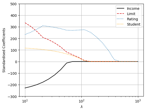
We can see that as \(\lambda\) increases, more and more of the coefficient estimates are driven towards zero. This is a consequence of the \(L_1\) penalty, which has the effect of forcing some of the coefficient estimates to be exactly equal to zero when the tuning parameter \(\lambda\) is sufficiently large. In this way, Lasso performs embedded feature selection, in addition to shrinking the coefficient estimates. In fact, Lasso will completely eliminate some of the features from the final model, which is not the case with ridge regression. This can be useful for interpretation.
As in the case of ridge regression, the tuning parameter \(\lambda\) must be chosen carefully. Let us study the test MSE corresponding to the various values of \(\lambda\).
mses = []

lambdas = np.logspace(-2, 2, 20)

for lambda_ in lambdas:
    lasso = Lasso(alpha=lambda_)
    lasso.fit(X_train, y_train)
    mses.append(mean_squared_error(y_test, lasso.predict(X_test)))

print("Best MSE: ", np.min(mses))

fig, ax = plt.subplots(figsize=(10, 6))

ax.plot(lambdas, mses, c="m", ls="-", label="$MSE(x)$")
ax.vlines(1, np.min(mses), np.max(mses), colors="k", ls="--", label="Optimal $\lambda$")

# add annotation
ax.annotate("Overfit (high variance, high bias)", xy=(0.01, 19000), fontsize=14)
ax.annotate(
    "",
    xy=(0.05, 14000),
    xytext=(0.05, 19000),
    arrowprops=dict(arrowstyle="->", relpos=(0, 0)),
)
ax.annotate(
    "Underfit (high bias, low variance)",
    xy=(70, 45000),
    xytext=(2, 55000),
    arrowprops=dict(arrowstyle="->"),
    fontsize=14,
)
ax.annotate("Optimal", xy=(5, 18000), fontsize=14)
ax.annotate(
    "",
    xy=(lambdas[np.argmin(mses)], np.min(mses)),
    xytext=(lambdas[np.argmin(mses)], 18000),
    arrowprops=dict(arrowstyle="->", relpos=(0, 0)),
)

plt.xscale("log")
plt.yscale("log")
plt.xlabel(r"$\lambda$")
plt.ylabel("Mean Squared Error")
plt.grid(True)
plt.show()
Best MSE: 12956.57245152192
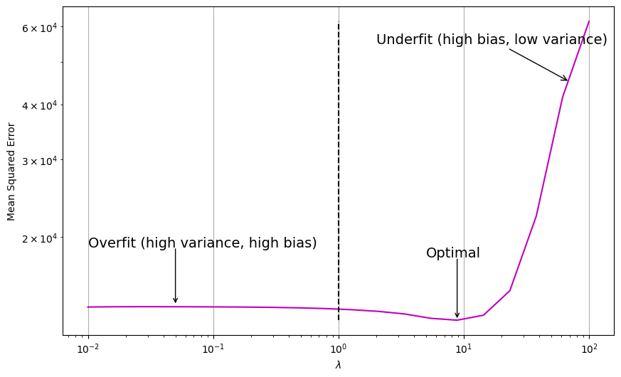
Here, we observe a similar pattern to that of ridge regression. As \(\lambda\) increases, the test MSE initially decreases and then increases again.
6.2.2.2. Another formulation of ridge regression and lasso
One can show that the lasso and ridge regression coefficient estimates solve the problems
and
respectively, where t is a threshold. Thus, the lasso and ridge regression solutions are the unique minimisers of the corresponding constrained optimisation problems with \(L_1\) and \(L_2\) constraints (penalties), respectively.
6.2.2.3. Feature selection property of the lasso

Fig. 6.1 Contours of the error and constraint functions for the lasso (left) and ridge regression (right). source: https://commons.wikimedia.org/wiki/File:Regularization.jpg
Why is it that the lasso, unlike ridge regression, results in coefficient estimates that are exactly equal to zero? The figure above illustrates the case when \(D=2\). The least squares solution is marked as \(\hat{\beta}\) while the blue diamond and circle represent the lasso and ridge regression constraints, respectively. If \(t\) is sufficiently large, then the constraint regions will contain \(\hat{\beta}\), and so the ridge regression and lasso estimates will be the same as the least squares estimates. (Such a large value of \(t\) corresponds to \(\lambda = 0 \) in Equation (6.2) and Equation (6.3).) However, in Fig. 6.1, \(t\) is not large enough so the least squares estimates lie outside of the diamond and the circle, and the least squares estimates are not the same as the lasso and ridge regression estimates.
Each of the ellipses centred around \(\hat{\beta}\) represents a contour: this means that all of the points on a particular ellipse have the same RSS value. As the ellipses expand away from the least squares coefficient estimates, the RSS increases. Equations (6.4) and (6.5) indicate that the lasso and ridge regression coefficient estimates are given by the first point at which an ellipse contacts the constraint region. Since ridge regression has a circular constraint with no sharp points, this intersection will not generally occur on an axis, and so the ridge regression coefficient estimates will be exclusively non-zero. However, the lasso constraint has corners at each of the axes, and so the ellipse will often intersect the constraint region at an axis. When this occurs, one of the coefficients will equal to zero. For example, in Fig. 6.1, the intersection occurs at \(\beta_1 = 0\), and so the resulting model will only include \(\beta_2\). In higher dimensions, many of the coefficient estimates may equal to zero simultaneously. This is the reason why the lasso results in some coefficient estimates that are exactly equal to zero.
6.2.3. Comparing the lasso and ridge regression
It is clear that the lasso has a major advantage over ridge regression, in that it produces simpler and more interpretable models that involve only a subset of the predictors. However, which method leads to better prediction accuracy? By comparing the test MSEs in Ridge regression and Lasso, we can see that the lasso leads to a similar behaviour to ridge regression, while the minimum MSE of ridge regression is slightly smaller than that of the lasso. However, if the response variable is only correlated with a small subset of the predictors, then the lasso will perform better than ridge regression. This is because the lasso will set the coefficients of the irrelevant predictors to zero, whereas ridge regression will shrink them towards zero but not set them exactly to zero. In this case, the lasso will perform better because it will result in a model that involves only the relevant predictors.
In general, one might expect the lasso to perform better in a setting where a relatively small number of predictors have substantial coefficients, and the remaining predictors have coefficients that are very small or equal to zero. Ridge regression will perform better when the response is a function of many predictors, all with coefficients of roughly equal size. However, the number of predictors that is related to the response is never known a priori for real datasets. A technique such as cross-validation can be used to determine which approach is better on a particular dataset.
6.2.4. Exercises
1. All the following exercises use the Carseats dataset to study feature selection on real-world data.
Load the Carseats dataset, convert the values of variables (predictors) from category to numbers, and inspect the first five rows. (Use \(2022\) as the random seed value)
# Write your code below to answer the question
Compare your answer with the reference solution below
import numpy as np
import pandas as pd

np.random.seed(2022)

carseat_url = "https://github.com/pykale/transparentML/raw/main/data/Carseats.csv"

carseat_df = pd.read_csv(carseat_url)
# converting categories
carseat_df["ShelveLoc"] = carseat_df["ShelveLoc"].factorize()[0]
carseat_df["Urban"] = carseat_df["Urban"].factorize()[0]
carseat_df["US"] = carseat_df["US"].factorize()[0]

carseat_df.head(5)
| Sales | CompPrice | Income | Advertising | Population | Price | ShelveLoc | Age | Education | Urban | US | |
|---|---|---|---|---|---|---|---|---|---|---|---|
| 0 | 9.50 | 138 | 73 | 11 | 276 | 120 | 0 | 42 | 17 | 0 | 0 |
| 1 | 11.22 | 111 | 48 | 16 | 260 | 83 | 1 | 65 | 10 | 0 | 0 |
| 2 | 10.06 | 113 | 35 | 10 | 269 | 80 | 2 | 59 | 12 | 0 | 0 |
| 3 | 7.40 | 117 | 100 | 4 | 466 | 97 | 2 | 55 | 14 | 0 | 0 |
| 4 | 4.15 | 141 | 64 | 3 | 340 | 128 | 0 | 38 | 13 | 0 | 1 |
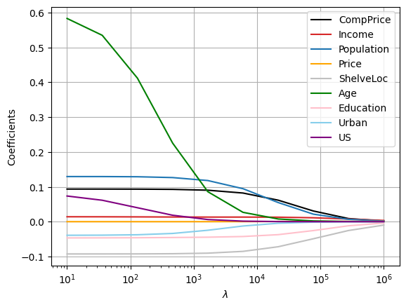
2. In continuation of Exercise 1, fit a ridge regression model using a set of \(10\) lambda values that are logarithmically spaced between \(1\) and \(6\). Plot the coefficient estimates for each lambda value and analyse which lambda value coefficient estimates are close to zero.
# Write your code below to answer the question
Compare your answer with the reference solution below
import matplotlib.pyplot as plt
from sklearn.linear_model import Ridge


X = carseat_df.drop(["Sales"], axis=1).values
y = carseat_df.Sales.values

lambdas = np.logspace(1, 6, 10)
coef_ridge = []

for lambda_ in lambdas:
    ridge = Ridge(alpha=lambda_)
    ridge.fit(X, y)
    coef_ridge.append(ridge.coef_)

coef_ridge = np.array(coef_ridge)
plt.plot(lambdas, coef_ridge[:, 0], c="black", label="CompPrice")
plt.plot(lambdas, coef_ridge[:, 1], c="tab:red", label="Income")
plt.plot(lambdas, coef_ridge[:, 2], c="tab:blue", label="Population")
plt.plot(lambdas, coef_ridge[:, 3], c="orange", label="Price")
plt.plot(lambdas, coef_ridge[:, 4], c="silver", label="ShelveLoc")
plt.plot(lambdas, coef_ridge[:, 5], c="green", label="Age")
plt.plot(lambdas, coef_ridge[:, 6], c="pink", label="Education")
plt.plot(lambdas, coef_ridge[:, 7], c="skyblue", label="Urban")
plt.plot(lambdas, coef_ridge[:, 8], c="purple", label="US")

plt.legend()
plt.xscale("log")

plt.xlabel(r"$\lambda$")
plt.ylabel("Coefficients")
plt.grid(True)
plt.show()
# We can observe that the coefficient estimates approach zero as the value of lambda increases.
# This is because the regularisation term in ridge regression has the effect of shrinking the coefficient estimates towards zero.
# The coefficient estimates for lambda values close to zero are very similar to the least squares estimates,
# whereas the coefficient estimates for lambda values close to 1000000 are very close to zero.
3. In continuation of Exercise 2, find the Mean Squared Errors (MSE) on the test data for all the lambda values and show the best MSE score.
# Write your code below to answer the question
Compare your answer with the reference solution below
from sklearn.model_selection import train_test_split
from sklearn.metrics import mean_squared_error

X_train, X_test, y_train, y_test = train_test_split(
    X, y, test_size=0.1, random_state=123, shuffle=True
)
# Define Algorithm

mses = []

lambdas = np.logspace(1, 6, 10)

for lambda_ in lambdas:
    ridge = Ridge(alpha=lambda_)
    ridge.fit(X_train, y_train)
    mses.append(mean_squared_error(y_test, ridge.predict(X_test)))

print("Best MSE: ", np.min(mses))
Best MSE: 2.3886905447334117
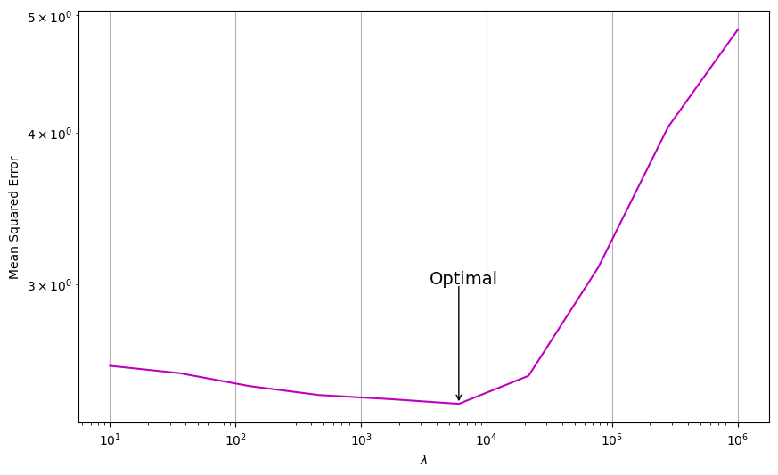
4. Plot the MSE scores for each lambda value and annotate the optimal point.
# Write your code below to answer the question
Compare your answer with the reference solution below
fig, ax = plt.subplots(figsize=(10, 6))

ax.plot(lambdas, mses, c="m", ls="-", label="$MSE(x)$")

# add annotation

ax.annotate("Optimal", xy=(3500, 3), fontsize=14)
ax.annotate(
    "",
    xy=(lambdas[np.argmin(mses)], np.min(mses)),
    xytext=(lambdas[np.argmin(mses)], 3),
    arrowprops=dict(arrowstyle="->", relpos=(0, 0)),
)

plt.xscale("log")
plt.yscale("log")
plt.xlabel(r"$\lambda$")
plt.ylabel("Mean Squared Error")
plt.grid(True)
plt.show()
5. The lasso, relative to least squares, is:
i. More flexible and hence will give improved prediction accuracy when its increase in bias is less than its decrease in variance.
   a. True

   b. False
Compare your answer with the solution below
b. False. Least squares uses all features, whereas lasso will either use all features or set coefficients to zero for some features. So lasso is either equivalent to least squares or less flexible.
ii. More flexible and hence will give improved prediction accuracy when its increase in variance is less than its decrease in bias.
   a. True

   b. False
Compare your answer with the solution below
b. False
iii. Less flexible and hence will give improved prediction accuracy when its increase in bias is less than its decrease in variance.
   a. True

   b. False
Compare your answer with the solution below
a. True. As \(\lambda\) (regularisation) is increased, the variance of the model will decrease quickly for a small increase in bias resulting in improved test MSE. At some point the bias will start to increase dramatically outweighing any benefits from further reduction in variance, at the expense of test MSE.
iv. Less flexible and hence will give improved prediction accuracy when its increase in variance is less than its decrease in bias.
   a. True

   b. False
Compare your answer with the solution below
b. False