Cross-validation
Contents
5.1. Cross-validation
Cross-validation is a resampling method that is commonly used to evaluate the performance of a machine learning model and subsequently select the appropriate level of flexibility of the given model or the best model from a set of candidate models. The process of evaluating a model’s performance is known as model assessment, whereas the process of selecting the proper level of flexibility for a model is known as model selection.
One round of cross-validation involves partitioning a sample of data into complementary subsets, performing the analysis on one subset (called the training set), and validating the analysis on the other subset (called the validation set or testing set). To reduce variability, multiple rounds of cross-validation are performed using different partitions, and the validation results are averaged over the rounds.
For example, a machine learning model may be evaluated by splitting the available data into a training set and a test set. The model is then trained on the training set, and its performance is measured on the test set. However, the evaluation procedure can have a high variance, depending on exactly which observations are included in the training set and which observations are included in the test set. Cross-validation remedies this problem by averaging the results over several complementary test sets and training sets. The method is called cross-validation because it involves training and testing the method on different subsets of the original data, where the subsets are different from each other in that the training sets are disjoint from the test sets. The method is also called rotation estimation because it can be thought of as a form of rotation among the available data.
Watch the 6-minute video below for a visual explanation of cross-validation:
Video
Explaining Cross Validation by StatQuest, embedded according to YouTube’s Terms of Service.
5.1.1. Import libraries and load data
Get ready by importing the APIs needed from respective libraries.
import pandas as pd
import numpy as np
import matplotlib.pyplot as plt
import seaborn as sns

from sklearn.linear_model import LinearRegression
from sklearn.metrics import mean_squared_error
from sklearn.model_selection import (
    train_test_split,
    LeaveOneOut,
    KFold,
    cross_val_score,
)
from sklearn.preprocessing import PolynomialFeatures

%matplotlib inline
Set a random seed for reproducibility.
np.random.seed(2022)
We will study cross-validation on the Auto dataset (click to explore). Load this dataset and inspect its structure (columns). Note here we remove entries with missing values using the dropna() function from the pandas library, which is a typical data cleaning step.
auto_url = "https://github.com/pykale/transparentML/raw/main/data/Auto.csv"

auto_df = pd.read_csv(auto_url, na_values="?").dropna()
auto_df.info()
<class 'pandas.core.frame.DataFrame'>
Index: 392 entries, 0 to 396
Data columns (total 9 columns):
 #   Column        Non-Null Count  Dtype
---  ------        --------------  -----
 0   mpg           392 non-null    float64
 1   cylinders     392 non-null    int64
 2   displacement  392 non-null    float64
 3   horsepower    392 non-null    float64
 4   weight        392 non-null    int64
 5   acceleration  392 non-null    float64
 6   year          392 non-null    int64
 7   origin        392 non-null    int64
 8   name          392 non-null    object
dtypes: float64(4), int64(4), object(1)
memory usage: 30.6+ KB
As usual, it is a good practice to inspect the first few rows before proceeding to any analysis.
auto_df.head()
| mpg | cylinders | displacement | horsepower | weight | acceleration | year | origin | name | |
|---|---|---|---|---|---|---|---|---|---|
| 0 | 18.0 | 8 | 307.0 | 130.0 | 3504 | 12.0 | 70 | 1 | chevrolet chevelle malibu |
| 1 | 15.0 | 8 | 350.0 | 165.0 | 3693 | 11.5 | 70 | 1 | buick skylark 320 |
| 2 | 18.0 | 8 | 318.0 | 150.0 | 3436 | 11.0 | 70 | 1 | plymouth satellite |
| 3 | 16.0 | 8 | 304.0 | 150.0 | 3433 | 12.0 | 70 | 1 | amc rebel sst |
| 4 | 17.0 | 8 | 302.0 | 140.0 | 3449 | 10.5 | 70 | 1 | ford torino |
5.1.2. Validation set approach
The validation set approach is a strategy to estimate the test error associated with fitting a particular model on a set of observations. It involves randomly dividing the available set of observations into two parts, a training set and a validation set or hold-out set. The model is fit on the training set, and the fitted model is used to predict the responses for the “unseen” (hold-out) observations in the validation set. The resulting validation set error rate, e.g. mean squared error (MSE) for a quantitative response, provides an estimate of the test error rate.
In the following example, we study linear regression on the Auto dataset. In Linear regression, we discovered a nonlinear relationship between mpg and horsepower. Compared to using only a linear term, a model that using horsepower and horsepower\(^2\) gives better results in predicts mpg. Can we tell what kind of nonlinear relationship between mpg and horsepower will give the best prediction performance?
We will use the validation set approach to estimate the test errors associated with different degrees (1 to 10) of polynomial expansion capturing different nonlinear relationships. We can randomly split the 392 observations of the Auto dataset into two sets, a training set containing 196 of the data points for model training, and a validation set containing the remaining 196 observations for evaluating by MSE. We will use the train_test_split() function from the sklearn.model_selection library to randomly split the data into two sets.
t_prop = 0.5
p_order = np.arange(1, 11)
r_state = np.arange(0, 10)

X, Y = np.meshgrid(p_order, r_state, indexing="ij")
Z = np.zeros((p_order.size, r_state.size))

regr = LinearRegression()

# Generate 10 random splits of the dataset
for (i, j), v in np.ndenumerate(Z):
    poly = PolynomialFeatures(int(X[i, j]))
    X_poly = poly.fit_transform(auto_df.horsepower.values.reshape(-1, 1))

    X_train, X_test, y_train, y_test = train_test_split(
        X_poly, auto_df.mpg.ravel(), test_size=t_prop, random_state=Y[i, j]
    )

    regr.fit(X_train, y_train)
    pred = regr.predict(X_test)
    Z[i, j] = mean_squared_error(y_test, pred)

fig, (ax1, ax2) = plt.subplots(1, 2, figsize=(10, 4))

# Left plot (first split)
ax1.plot(X.T[0], Z.T[0], "-o")
ax1.set_title("Random split of the dataset")

# Right plot (all splits)
ax2.plot(X, Z)
ax2.set_title("10 random splits of the dataset")

for ax in fig.axes:
    ax.set_ylabel("Mean Squared Error")
    ax.set_ylim(15, 30)
    ax.set_xlabel("Degree of Polynomial")
    ax.set_xlim(0.5, 10.5)
    ax.set_xticks(range(2, 11, 2));
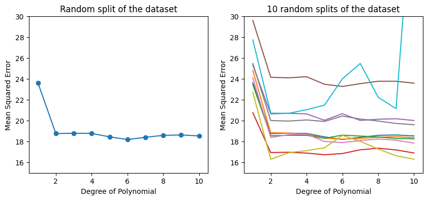
The left-hand panel of the figure above shows the results on one possible split of the data into a training set and a validation set using the polynomial regression model of different degrees. The training set is used to fit the model, and the validation set is used to evaluate the model fit. The validation set error rate is an estimate of the test error rate. The validation set error is lowest when the model is a function of horsepower\(^6\) in this case. Is this really/always the case?
If we repeat the process of randomly splitting, we will get a somewhat different estimate for the test MSE. Ten different validation set MSE curves are shown in the right-hand panel of the figure above.
We can observe:
model with a quadratic term has a dramatically smaller validation set MSE than the model with only a linear term
not much benefit in including cubic or higher-order polynomial terms in the model
each of the ten curves results in a different test MSE estimate for each of the ten regression models considered
there is no consensus among the curves as to which model results in the smallest validation set MSE.
Based on the variability among these curves, all that we can conclude with any confidence is that the linear fit is not adequate for this data. The validation set approach is conceptually simple and is easy to implement. But it has two drawbacks:
As is shown in the right-hand panel of the Figure above, the validation estimate of the test error rate can be highly variable, depending on precisely which observations are included in the training set and which observations are included in the validation set.
In the validation approach, only a subset of the observations—those that are included in the training set rather than in the validation set—are used to fit the model. Since machine learning models tend to perform worse when trained on fewer observations, this suggests that the validation set error rate may tend to overestimate the test error rate for the model fit on the entire dataset.
Cross-validation below is a refinement of the validation set approach that addresses these two issues.
5.1.3. Leave-one-out cross-validation
Leave-one-out cross-validation (LOOCV) is closely related to the validation set approach. It also splits the set of observations into two parts. However, instead of creating two subsets of comparable size, a single observation \((\mathbf{x}_i , y_i)\), where \( i = 1, 2, \cdots, N \), is used for the validation set, and the remaining observations \(\{(\mathbf{x}_1, y_1), (\mathbf{x}_2, y_2), \cdots, (\mathbf{x}_{i-1}, y_{i-1}), (\mathbf{x}_{i+1}, y_{i+1}), \cdots, (\mathbf{x}_N , y_N)\}\) make up the training set. The machine learning model is fit on the \( N − 1 \) training observations, and a prediction \(\hat{y}_i\) is made for the excluded observation, using its value \(\mathbf{x}_i\). Since \((\mathbf{x}_i , y_i)\) was not used in the fitting process, the squared test error \( \epsilon_i = (y_i − \hat{y}_i)^2 \) provides an approximately unbiased estimate.
We can repeat the procedure by iterating \(i\) from \(1\) to \(N\) to produce \(N\) squared errors, \( \epsilon_i, \dots, \epsilon_N \). The LOOCV estimate for the test MSE is the average of these \(N\) test error estimates:
Compared to the validation set approach, LOOCV has the following advantages:
LOOCV has far less bias. In LOOCV, we repeatedly fit the machine learning model using training sets that contain \(N − 1\) observations, almost as many as are in the entire dataset. This is in contrast to the validation set approach, in which the training set is typically around half the size of the original dataset. Consequently, the LOOCV approach tends not to overestimate the test error rate as much as the validation set approach does.
In contrast to the validation set approach which will yield different results when applied repeatedly due to randomness in the training/validation set splits, performing LOOCV multiple times will always yield the same results: there is no randomness in the training/validation set splits.
5.1.4. \(K\)-fold cross-validation
An alternative to LOOCV is \(K\)-fold CV. This approach involves randomly dividing the set of observations into \(K\) groups, or folds, of approximately equal size. Then repeating the following procedure by iterating \(k\) from \(1\) to \(K\):
Treating \(k\text{th}\) group of observations (fold) as a validation set,
Fitting model on the remaining \(K − 1\) folds,
Computing the mean squared error, \(\textrm{MSE}_k\)
This process results in \(K\) estimates of the test error, \(\textrm{MSE}_1, \textrm{MSE}_2, \dots, \textrm{MSE}_K\) . The \(K\)-fold CV estimate is computed by averaging these values,
LOOCV can be viewed as a special case of \(K\)-fold CV in which \(K = N\). In practice, one typically performs \(K\)-fold CV using \(K = 5\) or \(K = 10\). The most obvious advantage is computational. LOOCV requires fitting the machine learning model \(N\) times. This has the potential to be computationally expensive so may be feasible only for computationally efficient models. But cross-validation is a very general approach that can be applied to almost any machine learning model. Some machine learning models have computationally intensive fitting procedures, and so performing LOOCV may pose computational problems, especially if \(N\) is extremely large. In contrast, performing 10-fold CV requires fitting the learning procedure only ten times, which may be much more feasible.
Let us perform LOOCV on the Auto dataset. We will use the sklearn.model_selection module to perform the cross-validation. The cross_val_score function performs cross-validation for a given machine learning model.
p_order = np.arange(1, 11)
r_state = np.arange(0, 10)

# LeaveOneOut CV
regr = LinearRegression()
loo = LeaveOneOut()
loo.get_n_splits(auto_df)
scores = list()

for i in p_order:
    poly = PolynomialFeatures(i)
    X_poly = poly.fit_transform(auto_df.horsepower.values.reshape(-1, 1))
    score = cross_val_score(
        regr, X_poly, auto_df.mpg, cv=loo, scoring="neg_mean_squared_error"
    ).mean()
    scores.append(score)
Next, perform a 10-fold cross-validation (CV) using the same cross_val_score function from the sklearn.model_selection module, but this time using the cv=10 argument instead of cv=loo above.
# $10$-fold CV
folds = 10
elements = len(auto_df.index)

X, Y = np.meshgrid(p_order, r_state, indexing="ij")
Z = np.zeros((p_order.size, r_state.size))

regr = LinearRegression()

for (i, j), v in np.ndenumerate(Z):
    poly = PolynomialFeatures(X[i, j])
    X_poly = poly.fit_transform(auto_df.horsepower.values.reshape(-1, 1))
    kf_10 = KFold(n_splits=folds, random_state=Y[i, j], shuffle=True)
    Z[i, j] = cross_val_score(
        regr, X_poly, auto_df.mpg, cv=kf_10, scoring="neg_mean_squared_error"
    ).mean()
Let us compare the results of the LOOCV and 10-fold CV.
fig, (ax1, ax2) = plt.subplots(1, 2, figsize=(10, 4))

# Note: cross_val_score() method return negative values for the scores.
# https://github.com/scikit-learn/scikit-learn/issues/2439

# Left plot
ax1.plot(p_order, np.array(scores) * -1, "-o")
ax1.set_title("LOOCV")

# Right plot
ax2.plot(X, Z * -1)
ax2.set_title("10-fold CV")

for ax in fig.axes:
    ax.set_ylabel("Mean Squared Error")
    ax.set_ylim(15, 30)
    ax.set_xlabel("Degree of Polynomial")
    ax.set_xlim(0.5, 10.5)
    ax.set_xticks(range(2, 11, 2));
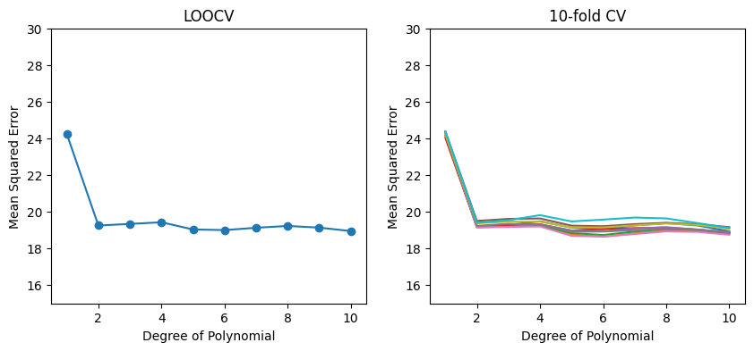
The results of LOOCV and 10-fold CV are shown in the left and right panels, respectively. As we can see from the figure, there is some variability in the 10-fold CV estimates as a result of the variability in how the observations are divided into ten folds. But this variability is typically much lower than the variability in the test error estimates that results from the validation set approach.
The objective of performing cross-validation can be different:
For model evaluation, our goal might be to determine how well a given machine learning model can be expected to perform on independent data; in this case, the actual estimate of the test MSE is of interest.
For model selection, we are interested only in the location of the minimum point in the estimated test MSE curve. This is because we might be performing cross-validation on a number of machine learning models, or on a single model using different levels of flexibility (typically different hyper-parameters), in order to identify the model that results in the lowest test error. For this purpose, the location of the minimum point in the estimated test MSE curve is important, but the actual value of the estimated test MSE is not.
You can explore further by learning from the cross-validation strategies in scikit-learn.
5.1.5. Exercises
1. Explain how \(K\)-fold cross-validation is implemented.
Compare your answer with the solution below
In \(K\)-fold cross validation, the original set of observations are randomly divided into \(K\) equal sized folds (groups). Of the \(K\) folds, a single fold is retained as the validation data for testing the model, and the remaining \(K − 1\) folds are used as training data. The cross-validation process is then repeated \(K\) times, with each of the \(K\) folds used exactly once as the validation data. The \(K\) results can then be averaged to produce a single estimation.
2. In Chapter 3, we used logistic regression on the Default dataset to predict the probability of someone defaulting on a loan, by looking at their income and balance. We will now estimate the test error of this logistic regression model using the validation set approach. Do not forget to set a random seed before beginning your analysis and convert the categories to numerical values.
a. Fit a logistic regression model that uses income and balance to predict default and uses the validation set approach to estimate the test error of this model. In order to do this, you must perform the following steps:
i. Split the sample set into a training set and a validation set.
ii. Fit a multiple logistic regression model using only the training observations.
iii. Obtain a prediction of default status for each individual in the validation set.
iv. Compute the validation set error, which is the fraction of the observations in the validation set that are misclassified. Hint: See section 5.1.2.
# Write your code below to answer the question
Compare your answer with the reference solution below
import numpy as np
import pandas as pd
import matplotlib.pyplot as plt
import seaborn as sns
from sklearn.linear_model import LogisticRegression
from sklearn.model_selection import train_test_split
from sklearn.metrics import mean_squared_error

default_df = pd.read_csv(
    "https://github.com/pykale/transparentML/raw/main/data/Default.csv"
)

# Check for missing
assert default_df.isna().sum().sum() == 0

# converting categories
default_df["default"] = default_df.default.factorize()[0]
default_df["student"] = default_df.student.factorize()[0]

np.random.seed(1)

X = default_df[["income", "balance"]].values
Y = default_df["default"]

# train test spliting 50:50
X_train, X_test, y_train, y_test = train_test_split(X, Y.ravel(), test_size=0.5)

# Logistic regression
logit = LogisticRegression()
model_logit = logit.fit(X_train, y_train)

# Predict
y_pred = model_logit.predict(X_test)

total_error_rate_pct = mean_squared_error(y_test, y_pred) * 100
print("total_error_rate: {}%".format(total_error_rate_pct))
total_error_rate: 3.2199999999999998%
b. Repeat the process in Exercise 2(a) three times, using three different splits of the observations into a training set and a validation set. Comment on the results obtained. Hint: Try using different random seed values.
# Write your code below to answer the question
Compare your answer with the reference solution below
for s in range(1, 4):
    print("Random seed = {}".format(s))
    np.random.seed(s)
    X_train, X_test, y_train, y_test = train_test_split(X, Y.ravel(), test_size=0.5)

    # Logistic regression
    logit = LogisticRegression()
    model_logit = logit.fit(X_train, y_train)

    # Predict
    y_pred = model_logit.predict(X_test)

    total_error_rate_pct = mean_squared_error(y_test, y_pred) * 100
    print("total_error_rate: {}%".format(total_error_rate_pct))

# For different seed value we gets different error rate as our train_test_split is random. We can use random state parameter inside the train_test)split also to control the randomness
Random seed = 1
total_error_rate: 3.2199999999999998%
Random seed = 2
total_error_rate: 3.1199999999999997%
Random seed = 3
total_error_rate: 3.4000000000000004%
c. Again, consider a logistic regression model that predicts the probability of default using income, balance, and a dummy variable for student. Estimate the test error for this model using the validation set approach. Comment on whether or not including a dummy variable for student leads to a reduction in the test error rate.
# Write your code below to answer the question
Compare your answer with the reference solution below
X = default_df[["income", "balance", "student"]].values
Y = default_df["default"]

for s in range(1, 4):
    print("Random seed = {}".format(s))
    np.random.seed(s)
    X_train, X_test, y_train, y_test = train_test_split(X, Y.ravel(), test_size=0.5)

    # Logistic regression
    logit = LogisticRegression()
    model_logit = logit.fit(X_train, y_train)
    # Predict
    y_pred = model_logit.predict(X_test)
    total_error_rate_pct = mean_squared_error(y_test, y_pred) * 100
    print("total_error_rate: {}%".format(total_error_rate_pct))


# Including a dummy variable for student didn't leads to a reduction in the test error rate.
Random seed = 1
total_error_rate: 3.2199999999999998%
Random seed = 2
total_error_rate: 3.2%
Random seed = 3
total_error_rate: 3.4000000000000004%
d. Fit a logistic regression model that uses income and balance to predict default by performing leave-one-out cross-validation and \(5\)-fold cross-validation to estimate the test error. For simplicity, use the first \(1000\) samples from the dataset to perform this experiment. Hint: See section 5.1.3 and 5.1.4.
# Write your code below to answer the question
Compare your answer with the reference solution below
from sklearn.model_selection import (
    LeaveOneOut,
    KFold,
    cross_val_score,
)

df = default_df[:1000]

X = df[["income", "balance"]].values
Y = df["default"]

regr = LogisticRegression()
# LeaveOneOut CV
loo = LeaveOneOut()
loo.get_n_splits(default_df)

loocv_score = cross_val_score(
    regr, X, Y, cv=loo, scoring="neg_mean_squared_error"
).mean()

# 5-fold CV
folds = 5
kf_5 = KFold(n_splits=folds, shuffle=True)
kf_score = cross_val_score(regr, X, Y, cv=kf_5, scoring="neg_mean_squared_error").mean()
print("total_error_rate for loocv: {}%".format(-1 * loocv_score * 100))
print("total_error_rate for 5-Fold: {}%".format(-1 * kf_score * 100))

# Test error for loocv is lower then the 5-fold cross validation
total_error_rate for loocv: 2.5%
total_error_rate for 5-Fold: 3.0000000000000004%