Ensemble learning
Contents
7.3. Ensemble learning
As mentioned in the previous sections, fitting a single decision tree, a regression/classification tree, to a dataset is prone to overfitting. To overcome this problem, we can use ensemble learning methods, which combine multiple simple “building block” models such as decision trees to produce a single, potentially more powerful model for a single consensus prediction. These simple building block models are called “weak learners” so an ensemble learning method aim to leverage many weak learners to produce a single strong learner that is less prone to overfitting and has better predictive power. However, ensemble learning methods are more difficult to interpret than single decision trees.
In this section, we will study three ensemble learning methods that use decision trees as building blocks: bagging, random forests, and boosting.
Watch the 9-minute video below for a visual explanation of random forests.
Video
Explaining Random Forests by StatQuest, embedded according to YouTube’s Terms of Service.
7.3.1. Bagging
Bagging stands for “bootstrap aggregating”. It is a general ensemble learning method that can be used with any model, not just decision trees. The idea is to fit multiple copies of the same model to different subsets of the data, and then combine the predictions of all the models to produce a single consensus prediction. The subsets of the data are sampled with replacement, which means that some observations may be sampled more than once, and some observations may not be sampled at all. This is called “bootstrapping”, covered earlier in Chapter 5). The term “aggregating” refers to the fact that the predictions of all the models are combined to produce a single consensus prediction.
Decision trees suffer from high variance. If we split the training data into two subsets, and fit a decision tree to each subset, the two trees will be very different. Bagging reduces the variance of a single decision tree by fitting \(B\) regression/classification trees to \(B\) bootstrapped training sets, sampled with replacement from the original training set. The predictions of all the \(B\) trees are then combined to produce a single consensus prediction. The consensus prediction is the average of the predictions of all the \(B\) trees for regression trees, and the majority vote of the predictions of all the \(B\) trees for classification trees.
7.3.1.1. Out-of-bag (OOB) error
In bagging, each bootstrap sample is sampled with replacement from the original training set. This means that some observations may not be sampled at all in a bootstrap sample. These observations are called “out-of-bag” (OOB) observations. The predictions of the \(B\) trees for the OOB observations are then used to estimate the OOB error. The OOB error is a good estimate of the test error, and can be used to tune the hyperparameters of the model. With \(B\) sufficiently large, the OOB error is virtually equivalent to leave-one-out cross-validation error.
7.3.1.2. Feature importance measures
Bagging typically leads to a better predictive performance than a single decision tree. However, the resulting model is more difficult to interpret than a single decision tree. One way to interpret the bagging model is to look at the average feature importance measures across all the \(B\) trees, where the feature importance measures of a single decision tree are the average decrease in the cost function, e.g. the mean squared error for regression trees, and the Gini index for classification trees.
Bagging is a very simple ensemble learning method that is easy to implement and understand. However, it is not as powerful as random forests and boosting, which we will discuss next.
7.3.2. Random forests
Random forests is a popular ensemble learning method that uses decision trees as building blocks. It is a generalization of bagging that uses a slightly different approach to combine the predictions of the \(B\) trees. It still fits \(B\) regression/classification trees to \(B\) bootstrapped training sets, sampled with replacement from the original training set. However, instead of using all the \(D\) features to fit each tree, random forests use a random subset of the \(D\) features to fit each tree. This is called “feature bagging”. The number of features to use in each tree is typically chosen to be \(\sqrt{D}\), where \(D\) is the total number of features. In this way, random forests decorrelates the trees, which reduces the variance of the ensemble learning method.
The building blocks of random forests are weaker learners than the building blocks of bagging, but the resulting model is more powerful, due to the decorrelation of the trees and the resulting diversity that enables the model to capture more complementary information from the data.
7.3.3. Boosting
Boosting is another popular ensemble learning method that can use any model as building blocks, though we will consider only decision trees here. It is another generalization of bagging that uses a slightly different approach to combine the predictions of the \(B\) trees. It still fits \(B\) regression/classification trees to \(B\) bootstrapped training sets, sampled with replacement from the original training set. However, instead of fitting each tree independently, boosting fits each tree sequentially, where each tree is fit to the residuals of the previous tree. This is called “boosting”.
The first tree is fit to the original training data, and each subsequent tree is fit to a modified version of the training data. The modification of the training data is done by assigning a weight to each observation in the training data, and then fitting the tree to the training data using these weights. The weights are updated after each tree is fit, so that the subsequent trees are fit to the training data that are more difficult to predict, i.e. focusing on the challenging samples that are harder to predict at the current stage of the boosting process. The predictions of all the trees are then combined to produce a single consensus prediction.
Boosting is a powerful ensemble learning method that can be used to fit very accurate models. However, it is more difficult to implement and interpret than bagging and random forests.
7.3.4. Ensembles for income prediction
Let’s apply bagging, random forests, and boosting to the Boston dataset for regression.
Import the APIs and set a random seed for reproducibility.
import numpy as np
import pandas as pd
from math import sqrt
from sklearn.model_selection import train_test_split
from sklearn.tree import DecisionTreeRegressor
from sklearn.ensemble import (
    BaggingRegressor,
    GradientBoostingRegressor,
    RandomForestRegressor,
)
from sklearn.metrics import mean_squared_error

%matplotlib inline

np.random.seed(2022)  # set random seed for reproducibility
7.3.4.1. Compare the performance of bagging, random forests, and boosting
Load the Boston dataset and split it into training and test sets.
boston_url = "https://github.com/pykale/transparentML/raw/main/data/Boston.csv"
boston_df = pd.read_csv(boston_url)
X = boston_df.drop("medv", axis=1)
y = boston_df.medv
train_size = 0.5
max_depth = 3
X_train, X_test, y_train, y_test = train_test_split(X, y, train_size=train_size)
Apply bagging, random forests, and boosting to the Boston dataset for regression.
num_features = X.shape[1]
regr_bagging = BaggingRegressor(
base_estimator=DecisionTreeRegressor(max_depth=max_depth),
n_estimators=1000,
max_features=num_features,
bootstrap=True,
)
regr_bagging.fit(X_train, y_train)
y_pred_bagging = regr_bagging.predict(X_test)
mse_bagging = mean_squared_error(y_test, y_pred_bagging)
max_features = int(sqrt(num_features))
regr_rf = RandomForestRegressor(max_features=max_features)
regr_rf.fit(X_train, y_train)
y_pred_rf = regr_rf.predict(X_test)
mse_rf = mean_squared_error(y_test, y_pred_rf)
regr_boosting = GradientBoostingRegressor()
regr_boosting.fit(X_train, y_train)
y_pred_boosting = regr_boosting.predict(X_test)
mse_boosting = mean_squared_error(y_test, y_pred_boosting)
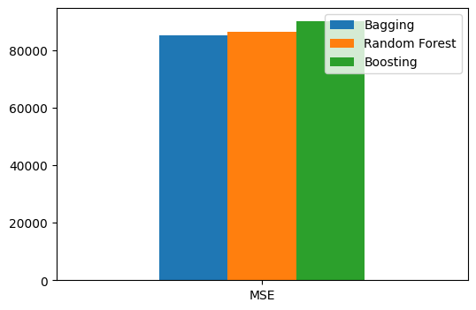
print("MSE for Bagging: {:.2f}".format(mse_bagging))
print("MSE for Random Forest: {:.2f}".format(mse_rf))
print("MSE for Boosting: {:.2f}".format(mse_boosting))
mses = pd.DataFrame(
{"Bagging": mse_bagging, "Random Forest": mse_rf, "Boosting": mse_boosting},
index=["MSE"],
)
mses.plot.bar(rot=0, figsize=(6, 4))
/opt/hostedtoolcache/Python/3.8.18/x64/lib/python3.8/site-packages/sklearn/ensemble/_base.py:156: FutureWarning: `base_estimator` was renamed to `estimator` in version 1.2 and will be removed in 1.4.
  warnings.warn(
MSE for Bagging: 16.26
MSE for Random Forest: 15.01
MSE for Boosting: 12.58
<Axes: >
7.3.4.2. Examine feature importance
Let us examine the feature importance for random forests and boosting.
rf_importances = regr_rf.feature_importances_
rf_indices = np.argsort(rf_importances)[::-1]
rf_names = [X.columns[i] for i in rf_indices]

boosting_importances = regr_boosting.feature_importances_
boosting_indices = np.argsort(boosting_importances)[::-1]
boosting_names = [X.columns[i] for i in boosting_indices]

importances = pd.DataFrame(
    {
        "feature": X.columns,
        "Random Forest": rf_importances,
        "Boosting": boosting_importances,
    }
)
importances = importances.set_index("feature")
sorted_importances = importances.sort_values(by="Random Forest", ascending=False)
sorted_importances.plot.bar(rot=30, figsize=(10, 5))
<Axes: xlabel='feature'>
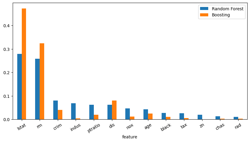
We can see that random forests and boosting agree on the top two most important features, i.e. LSTAT and RM, but the level of importance is different. Also, they start to disagree on which features are the next most important features from the third most important feature onwards. Random forests consider CRIM to be the third most important feature, while boosting considers DIS to be the third most important feature.
7.3.5. Exercises
1. All the following exercises use the Hitters dataset.
Load the Hitters dataset, convert the values of variables (predictors) from categorical values to numerical values, and inspect the first five rows.
# Write your code below to answer the question
Compare your answer with the reference solution below
import numpy as np
import pandas as pd
from sklearn.model_selection import train_test_split

np.random.seed(2022)  # set random seed for reproducibility

hitters_url = "https://github.com/pykale/transparentML/raw/main/data/Hitters.csv"
hitters_df = pd.read_csv(hitters_url).dropna()
hitters_df["League"] = hitters_df["League"].factorize()[0]
hitters_df["Division"] = hitters_df["Division"].factorize()[0]
hitters_df["NewLeague"] = hitters_df["NewLeague"].factorize()[0]

hitters_df.head()
| AtBat | Hits | HmRun | Runs | RBI | Walks | Years | CAtBat | CHits | CHmRun | CRuns | CRBI | CWalks | League | Division | PutOuts | Assists | Errors | Salary | NewLeague | |
|---|---|---|---|---|---|---|---|---|---|---|---|---|---|---|---|---|---|---|---|---|
| 1 | 315 | 81 | 7 | 24 | 38 | 39 | 14 | 3449 | 835 | 69 | 321 | 414 | 375 | 0 | 0 | 632 | 43 | 10 | 475.0 | 0 |
| 2 | 479 | 130 | 18 | 66 | 72 | 76 | 3 | 1624 | 457 | 63 | 224 | 266 | 263 | 1 | 0 | 880 | 82 | 14 | 480.0 | 1 |
| 3 | 496 | 141 | 20 | 65 | 78 | 37 | 11 | 5628 | 1575 | 225 | 828 | 838 | 354 | 0 | 1 | 200 | 11 | 3 | 500.0 | 0 |
| 4 | 321 | 87 | 10 | 39 | 42 | 30 | 2 | 396 | 101 | 12 | 48 | 46 | 33 | 0 | 1 | 805 | 40 | 4 | 91.5 | 0 |
| 5 | 594 | 169 | 4 | 74 | 51 | 35 | 11 | 4408 | 1133 | 19 | 501 | 336 | 194 | 1 | 0 | 282 | 421 | 25 | 750.0 | 1 |
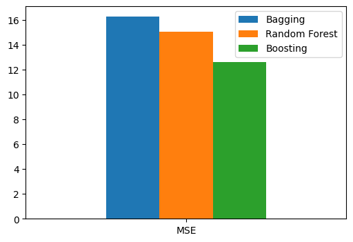
2. Train three models on the dataset loaded in Exercise 1 using the bagging, random forests, and boosting methods, and compare their performance on the test dataset using MSE as the evaluation metric.
# Write your code below to answer the question
Compare your answer with the reference solution below
from sklearn.tree import DecisionTreeRegressor
from sklearn.ensemble import (
    BaggingRegressor,
    GradientBoostingRegressor,
    RandomForestRegressor,
)
from sklearn.metrics import mean_squared_error
from math import sqrt

X = hitters_df.drop("Salary", axis=1)
y = hitters_df.Salary
train_size = 0.5
max_depth = 3
X_train, X_test, y_train, y_test = train_test_split(X, y, train_size=train_size)


num_features = X.shape[1]
regr_bagging = BaggingRegressor(
    base_estimator=DecisionTreeRegressor(max_depth=max_depth),
    n_estimators=1000,
    max_features=num_features,
    bootstrap=True,
)
regr_bagging.fit(X_train, y_train)
y_pred_bagging = regr_bagging.predict(X_test)
mse_bagging = mean_squared_error(y_test, y_pred_bagging)

max_features = int(sqrt(num_features))
regr_rf = RandomForestRegressor(max_features=max_features)
regr_rf.fit(X_train, y_train)
y_pred_rf = regr_rf.predict(X_test)
mse_rf = mean_squared_error(y_test, y_pred_rf)

regr_boosting = GradientBoostingRegressor()
regr_boosting.fit(X_train, y_train)
y_pred_boosting = regr_boosting.predict(X_test)
mse_boosting = mean_squared_error(y_test, y_pred_boosting)

print("MSE for Bagging: {:.2f}".format(mse_bagging))
print("MSE for Random Forest: {:.2f}".format(mse_rf))
print("MSE for Boosting: {:.2f}".format(mse_boosting))

mses = pd.DataFrame(
    {"Bagging": mse_bagging, "Random Forest": mse_rf, "Boosting": mse_boosting},
    index=["MSE"],
)
mses.plot.bar(rot=0, figsize=(6, 4))
/opt/hostedtoolcache/Python/3.8.18/x64/lib/python3.8/site-packages/sklearn/ensemble/_base.py:156: FutureWarning: `base_estimator` was renamed to `estimator` in version 1.2 and will be removed in 1.4.
  warnings.warn(
MSE for Bagging: 85200.41
MSE for Random Forest: 86194.81
MSE for Boosting: 90029.64
<Axes: >
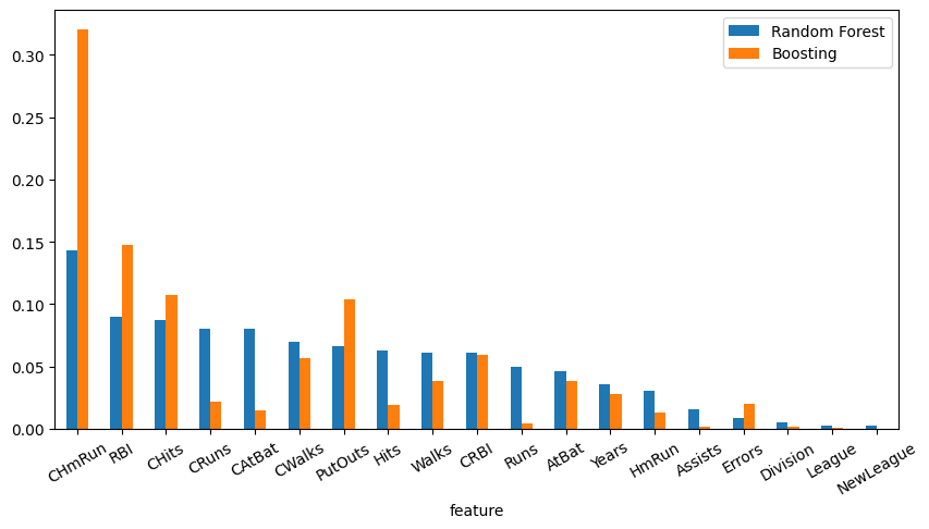
3. Find and compare the important features of the random forest and boosting models.
# Write your code below to answer the question
Compare your answer with the reference solution below
rf_importances = regr_rf.feature_importances_
boosting_importances = regr_boosting.feature_importances_
boosting_indices = np.argsort(boosting_importances)[::-1]
boosting_names = [X.columns[i] for i in boosting_indices]


importances = pd.DataFrame(
    {
        "feature": X.columns,
        "Random Forest": rf_importances,
        "Boosting": boosting_importances,
    }
)
importances = importances.set_index("feature")
sorted_importances = importances.sort_values(by="Random Forest", ascending=False)
sorted_importances.plot.bar(rot=30, figsize=(10, 5))
<Axes: xlabel='feature'>