Principal component analysis
Contents
9.1. Principal component analysis
This section introduces principal component analysis (PCA). PCA is a popular method for reducing the dimensionality of data, often represented as a data matrix \(\mathbf{X} \in \mathbb{R}^{D \times N}\), where \(N\) is the number of observations and \(D\) is the number of variables (features). When faced with a large set of potentially correlated variables, PCA allows us to summarise this set with a smaller number of representative variables that collectively explain most of the variability in the original set.
PCA is an unsupervised method, since it involves only a set of \(D\) features \(x_1, \ldots, x_D\) and no associated response \(y\). PCA is a standard feature extraction or feautre/representation learning that is often used as a pre-processing step to reduce the feature dimensionality for supervised learning problems. PCA also serves as a standard tool for data visualisation, for visualising either observations or features. It can also be used as a factorisation model for data imputation, i.e. for filling in missing values in a data matrix.
Watch the 5-minute video below for a visual explanation of principal component analysis.
Video
Explaining main ideas behind principal component analysis by StatQuest, embedded according to YouTube’s Terms of Service.
9.1.1. PCA for dimensionality reduction
9.1.1.1. Motivation
Suppose that we wish to visualise observations with measurements on a set of \( D \) features, \(x_1, x_2, \ldots, x_D \), as part of an exploratory data analysis. We could do this by examining two-dimensional scatterplots of the data, each of which contains the \(N\) observations’ measurements on two of the features. However, there are \( D(D-1)/2 \) such scatterplots, and it is difficult to visualise more than a few of them at a time even for a \(D\) of small value (e.g. if \(D=10\), then \( D(D-1)/2 = 45 \)). If \( D \) is large, then it will certainly not be possible to look at all of them; moreover, most likely none of them will be informative since they each contain just a small fraction of the total information present in the dataset.
Clearly, a better method is needed to visualise the \(N\) observations when \(D\) is large. In particular, we would like to find a lower-dimensional representation of the data that captures as much of the information as possible. For instance, if we can obtain a two-dimensional representation of the data that captures most of the information, then we can plot the observations in this lower-dimensional space to gain a visual understanding of the data.
PCA provides a tool to do just this. It finds a lower-dimensional representation of a dataset that contains as much as possible of the variation. The idea is that each of the \(N\) observations lives in \(D\)-dimensional space, but not all of these dimensions are equally interesting. PCA seeks a small number of dimensions that are as interesting as possible, where the concept of interesting is measured by the amount that the observations vary along each dimension.
9.1.1.2. Principal components (PCs)
Each of the dimensions found by PCA is called a principal component (PC), and it is a linear combination of the \(D\) features.
The first PC of a set of features \(x_1, \ldots, x_D\) is the normalised linear combination of the features
that has the largest variance. By normalised, we mean that \( \sum_{d=1}^D \phi_{d,1}^2 = 1 \) for the first PC \(m=1\) and \( \sum_{d=1}^D \phi_{d,m}^2 = 1\) for the \(m\text{th}\) PC in general. We refer to the elements \(\phi_{1, 1}, \ldots, \phi_{D, 1} \) as the loadings of the first principal loading component. Together, the loadings make up the first principal component loading vector, \(\boldsymbol{\phi}_1 = [\phi_{1,1}, \ldots, \phi_{D,1}]^\top\). We constrain the loadings so that their sum of squares is equal to one, i.e. normalised, since otherwise setting these elements to be arbitrarily large in absolute value could result in an arbitrarily large variance, giving a trivial solution.
9.1.1.3. Computing the first PC
Given a \(D \times N\) dataset as a data matrix \(\mathbf{X}\), how do we compute the first principal component? Since we are only interested in variance, we assume that each of the features in \( \mathbf{X} \) has been centred to have mean zero (that is, the column means of \( \mathbf{X} \) are zero). We then look for the linear combination of the sample feature values of the form
that has the largest sample variance, subject to the constraint that \(\sum_{d=1}^D \phi_{d,1}^2 = 1\). In other words, the first principal component loading vector \(\boldsymbol{\phi}_1\) solves the optimisation problem
where the objective can also be written as \(\frac{1}{N} \sum_{n=1}^N y_{n,1}^2 \). Equation (9.1) maximises the sample variance of the \(N\) values of \( y_{n,1} \). We refer \( y_{1,1}, \ldots, y_{N,1} \) as the first principal component scores. Equation (9.1) can be solved via a standard technique in linear algebra, eigendecomposition or singular value decomposition, as the first eigenvector of the covariance matrix \(\mathbf{X}\mathbf{X}^\top\), the one corresponding to the largest eigenvalue, where this eigenvalue is the variance captured in \( \{y_{n,1}\}\). The mathematical details of which are beyond the scope of this course.
9.1.1.4. Interpreting the first PC
There is a nice geometric interpretation for the first principal component. The loading vector \( \boldsymbol{\phi}_1 \) with elements \( \phi_{1,1}, \ldots, \phi_{D, 1} \) defines a direction in feature space along which the data vary the most. If we project the \(N\) data points \(\mathbf{x}_1, \ldots, \mathbf{x}_N\) onto this direction, the projected values are the principal component scores \( y_{1, 1} , \ldots , y_{N, 1}\) themselves.
9.1.1.5. Computing the second PC and beyond
After the first principal component \( y_{n,1} \) of the features has been determined, we can find the second principal component \( y_{n,2} \). The second principal component is the linear combination of \( x_1 , \ldots, x_D \) that has maximal variance out of all linear combinations that are uncorrelated with \( y_1 \). The second principal component scores \( y_{1,2}, y_{2,2}, \ldots , y_{N,2}\) take the form
where \( \boldsymbol{\phi}_2 = [\phi_{1,2}, \ldots, \phi_{D,2}]^\top\) is the second principal component loading vector. It turns out that constraining \( \{y_{n,2}\} \) to be uncorrelated with \( \{y_{n,1}\} \) is equivalent to constraining the direction \( \boldsymbol{\phi}_2 \) to be orthogonal (perpendicular) to the direction \( \boldsymbol{\phi}_1 \). Thus, by (beautiful) linear algebra, \( \boldsymbol{\phi}_2 \) is the second eigenvector of the covariance matrix \(\mathbf{X}\mathbf{X}^\top\), the one corresponding to the second largest eigenvalue that equals to the variance captured in \( \{y_{n,2}\}\).
The following principal component loading vectors \( \boldsymbol{\phi}_3 \), \( \boldsymbol{\phi}_4 \), and so forth are the third, fourth, and so forth eigenvectors of the covariance matrix \(\mathbf{X}\mathbf{X}^\top\), the ones corresponding to the third, fourth, and so forth largest eigenvalues. The corresponding principal component scores are \( \{y_{n,3}\} \), \( \{y_{n,4}\} \), and so forth.
9.1.1.6. Visualising the principal components
Once we have computed the principal components, we can plot them against each other in order to produce lower-dimensional views of the data. For instance, we can plot the score vector \( \{y_{n,1}\} \) against \( \{y_{n,2}\} \), \( \{y_{n,1}\} \) against \( \{y_{n,3}\} \), \( \{y_{n,2}\} \) against \( \{y_{n,3}\} \), and so forth. Geometrically, this amounts to projecting the original data down onto the subspace spanned by \( \boldsymbol{\phi}_1 \), \( \boldsymbol{\phi}_2 \), and \( \boldsymbol{\phi}_3 \), and plotting the projected points.
Interactive exploration
You can explore PCA-based visualisation interactively in the Embedding Projector by TensorFlow, noting that the default visualisation algorithm is PCA and you can choose different principal components (up to three) to visualise.
9.1.1.7. PCA as the best low-rank approximation
The first \(M\) principal component score vectors and the first \(M\) principal component loading vectors provide the best \(M\)-dimensional (i.e. rank-\(M\)) approximation (in terms of Euclidean distance) to the \(n\text{th}\) observation \(\mathbf{x}_{n}\). This representation can be written in terms of the \(d\text{th}\) feature of \(\mathbf{x}_{n}\) as
When \(M\) is sufficiently large, the \(M\) principal component score vectors and \(M\) principal component loading vectors can give a good approximation to the data. When \(M = \min(N − 1, D)\), then the representation is exact: \(x_{n, d} = \sum_{m=1}^M \phi_{d, m} y_{n, m}\).
9.1.2. Analysing crimes in the US with PCA
We illustrate the use of PCA on the USArrests dataset. For each of the 50 states in the United States, the dataset contains the number of arrests per 100,000 residents for each of three crimes: Assault, Murder, and Rape. We also record UrbanPop (the percent of the population in each state living in urban areas). The principal component score vectors have length \(N = 50\), and the principal component loading vectors have length \(D = 4\). PCA was performed after standardizing each variable (feature) to have mean zero and standard deviation one.
Get ready by importing the APIs needed from respective libraries.
import pandas as pd
import numpy as np
from numpy.linalg import svd
import matplotlib as mpl
import matplotlib.pyplot as plt

from sklearn.preprocessing import StandardScaler
from sklearn.decomposition import PCA
from sklearn.cluster import KMeans
from scipy.cluster import hierarchy

%matplotlib inline
Load the data and print the first five rows.
data_url = "https://github.com/pykale/transparentML/raw/main/data/USArrests.csv"

USArrests = pd.read_csv(data_url, header=0, index_col=0)
USArrests.head()
| Murder | Assault | UrbanPop | Rape | |
|---|---|---|---|---|
| Alabama | 13.2 | 236 | 58 | 21.2 |
| Alaska | 10.0 | 263 | 48 | 44.5 |
| Arizona | 8.1 | 294 | 80 | 31.0 |
| Arkansas | 8.8 | 190 | 50 | 19.5 |
| California | 9.0 | 276 | 91 | 40.6 |
Inspect the mean and standard deviation of each feature.
print(USArrests.mean())
print(USArrests.var())
Murder        7.788
Assault     170.760
UrbanPop     65.540
Rape         21.232
dtype: float64
Murder        18.970465
Assault     6945.165714
UrbanPop     209.518776
Rape          87.729159
dtype: float64
Standardise the data by subtracting the mean and dividing by the standard deviation.
scaler = StandardScaler()
X = pd.DataFrame(
    scaler.fit_transform(USArrests), index=USArrests.index, columns=USArrests.columns
)
Perform PCA on the standardised data and print (all) the four principal component loading vectors.
# The loading vectors (i.e. these are the projection of the data onto the principal components)
pca_loadings = pd.DataFrame(
    PCA().fit(X).components_.T,
    index=USArrests.columns,
    columns=["V1", "V2", "V3", "V4"],
)
print(pca_loadings)
                V1        V2        V3        V4
Murder    0.535899  0.418181 -0.341233  0.649228
Assault   0.583184  0.187986 -0.268148 -0.743407
UrbanPop  0.278191 -0.872806 -0.378016  0.133878
Rape      0.543432 -0.167319  0.817778  0.089024
Use these principal component loading vectors to compute the principal component scores, i.e. transform the data to the principal component space.
pca = PCA()
df_plot = pd.DataFrame(
    pca.fit_transform(X), columns=["PC1", "PC2", "PC3", "PC4"], index=X.index
)
df_plot
| PC1 | PC2 | PC3 | PC4 | |
|---|---|---|---|---|
| Alabama | 0.985566 | 1.133392 | -0.444269 | 0.156267 |
| Alaska | 1.950138 | 1.073213 | 2.040003 | -0.438583 |
| Arizona | 1.763164 | -0.745957 | 0.054781 | -0.834653 |
| Arkansas | -0.141420 | 1.119797 | 0.114574 | -0.182811 |
| California | 2.523980 | -1.542934 | 0.598557 | -0.341996 |
| Colorado | 1.514563 | -0.987555 | 1.095007 | 0.001465 |
| Connecticut | -1.358647 | -1.088928 | -0.643258 | -0.118469 |
| Delaware | 0.047709 | -0.325359 | -0.718633 | -0.881978 |
| Florida | 3.013042 | 0.039229 | -0.576829 | -0.096285 |
| Georgia | 1.639283 | 1.278942 | -0.342460 | 1.076797 |
| Hawaii | -0.912657 | -1.570460 | 0.050782 | 0.902807 |
| Idaho | -1.639800 | 0.210973 | 0.259801 | -0.499104 |
| Illinois | 1.378911 | -0.681841 | -0.677496 | -0.122021 |
| Indiana | -0.505461 | -0.151563 | 0.228055 | 0.424666 |
| Iowa | -2.253646 | -0.104054 | 0.164564 | 0.017556 |
| Kansas | -0.796881 | -0.270165 | 0.025553 | 0.206496 |
| Kentucky | -0.750859 | 0.958440 | -0.028369 | 0.670557 |
| Louisiana | 1.564818 | 0.871055 | -0.783480 | 0.454728 |
| Maine | -2.396829 | 0.376392 | -0.065682 | -0.330460 |
| Maryland | 1.763369 | 0.427655 | -0.157250 | -0.559070 |
| Massachusetts | -0.486166 | -1.474496 | -0.609497 | -0.179599 |
| Michigan | 2.108441 | -0.155397 | 0.384869 | 0.102372 |
| Minnesota | -1.692682 | -0.632261 | 0.153070 | 0.067317 |
| Mississippi | 0.996494 | 2.393796 | -0.740808 | 0.215508 |
| Missouri | 0.696787 | -0.263355 | 0.377444 | 0.225824 |
| Montana | -1.185452 | 0.536874 | 0.246889 | 0.123742 |
| Nebraska | -1.265637 | -0.193954 | 0.175574 | 0.015893 |
| Nevada | 2.874395 | -0.775600 | 1.163380 | 0.314515 |
| New Hampshire | -2.383915 | -0.018082 | 0.036855 | -0.033137 |
| New Jersey | 0.181566 | -1.449506 | -0.764454 | 0.243383 |
| New Mexico | 1.980024 | 0.142849 | 0.183692 | -0.339534 |
| New York | 1.682577 | -0.823184 | -0.643075 | -0.013484 |
| North Carolina | 1.123379 | 2.228003 | -0.863572 | -0.954382 |
| North Dakota | -2.992226 | 0.599119 | 0.301277 | -0.253987 |
| Ohio | -0.225965 | -0.742238 | -0.031139 | 0.473916 |
| Oklahoma | -0.311783 | -0.287854 | -0.015310 | 0.010332 |
| Oregon | 0.059122 | -0.541411 | 0.939833 | -0.237781 |
| Pennsylvania | -0.888416 | -0.571100 | -0.400629 | 0.359061 |
| Rhode Island | -0.863772 | -1.491978 | -1.369946 | -0.613569 |
| South Carolina | 1.320724 | 1.933405 | -0.300538 | -0.131467 |
| South Dakota | -1.987775 | 0.823343 | 0.389293 | -0.109572 |
| Tennessee | 0.999742 | 0.860251 | 0.188083 | 0.652864 |
| Texas | 1.355138 | -0.412481 | -0.492069 | 0.643195 |
| Utah | -0.550565 | -1.471505 | 0.293728 | -0.082314 |
| Vermont | -2.801412 | 1.402288 | 0.841263 | -0.144890 |
| Virginia | -0.096335 | 0.199735 | 0.011713 | 0.211371 |
| Washington | -0.216903 | -0.970124 | 0.624871 | -0.220848 |
| West Virginia | -2.108585 | 1.424847 | 0.104775 | 0.131909 |
| Wisconsin | -2.079714 | -0.611269 | -0.138865 | 0.184104 |
| Wyoming | -0.629427 | 0.321013 | -0.240659 | -0.166652 |
Plot the first two principal component scores against each other for all 50 states. Also visualise the four principal component loading vectors.
fig, ax1 = plt.subplots(figsize=(9, 7))

ax1.set_xlim(-3.5, 3.5)
ax1.set_ylim(-3.5, 3.5)

# plot Principal Components 1 and 2
for i in df_plot.index:
    ax1.annotate(i, (df_plot.PC1.loc[i], -df_plot.PC2.loc[i]), ha="center")

# plot reference lines
ax1.hlines(0, -3.5, 3.5, linestyles="dotted", colors="grey")
ax1.vlines(0, -3.5, 3.5, linestyles="dotted", colors="grey")

ax1.set_xlabel("First Principal Component")
ax1.set_ylabel("Second Principal Component")

# plot Principal Component loading vectors, using a second y-axis.
ax2 = ax1.twinx().twiny()

ax2.set_ylim(-1, 1)
ax2.set_xlim(-1, 1)
ax2.tick_params(axis="y", colors="orange")
ax2.set_xlabel("Principal Component loading vectors", color="orange")

# plot labels for vectors. Variable 'a' is a small offset parameter to separate arrow tip and text.
a = 1.07
for i in pca_loadings[["V1", "V2"]].index:
    ax2.annotate(
        i, (pca_loadings.V1.loc[i] * a, -pca_loadings.V2.loc[i] * a), color="orange"
    )

# plot vectors
ax2.arrow(0, 0, pca_loadings.V1[0], -pca_loadings.V2[0])
ax2.arrow(0, 0, pca_loadings.V1[1], -pca_loadings.V2[1])
ax2.arrow(0, 0, pca_loadings.V1[2], -pca_loadings.V2[2])
ax2.arrow(0, 0, pca_loadings.V1[3], -pca_loadings.V2[3])
plt.show()
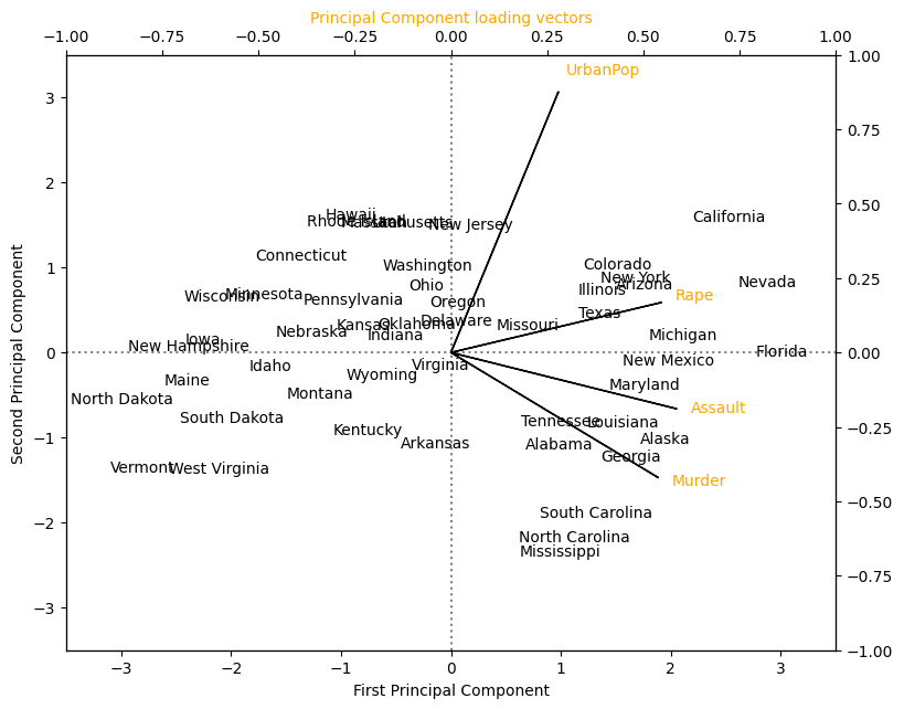
In the figure above, we can see that the first loading vector places approximately equal weight on Assault, Murder, and Rape, but with much less weight on UrbanPop. Hence this component roughly corresponds to a measure of overall rates of serious crimes. The second loading vector places most of its weight on UrbanPop and much less weight on the other three features. Hence, this component roughly corresponds to the level of urbanisation of the state. Overall, we see that the crime-related variables/features ( Murder, Assault, and Rape) are located close to each other, and that the UrbanPop variable/feature is far from the other three. This indicates that the crime-related variables are correlated with each other—states with high murder rates tend to have high assault and rape rates—and that the UrbanPop variable/feature is less correlated with the other three.
We can examine differences between the states via the two principal component score vectors shown in the figure above. Our discussion of the loading vectors suggests that states with large positive scores on the first component, such as California, Nevada and Florida, have high crime rates, while states like North Dakota, with negative scores on the first component, have low crime rates. California also has a high score on the second component, indicating a high level of urbanisation, while the opposite is true for states like Mississippi. States close to zero on both components, such as Indiana, have approximately average levels of both crime and urbanisation.
9.1.3. The proportion of variance explained
We can now ask a natural question: how much of the information in a given dataset is lost by projecting the observations onto the first \(M\) principal components? That is, how much of the variance in the data is not contained in the first \(M\) principal components? More generally, we are interested in knowing the proportion of variance explained (PVE) by each principal component. The total variance present in a dataset (assuming that the variables/features have been centred to have mean zero) is defined as
and the variance explained by the \(m\textrm{th}\) principal component is
Therefore, the PVE of the \(m\textrm{th}\) principal component is given by
The PVE of each principal component is a positive quantity. In order to compute the cumulative PVE of the first \(M\) principal components, we can simply sum Equation (9.2) over each of the first \(M\) PVEs. In total, there are (at most) \( \min (N − 1, D) \) principal components, and their PVEs sum to one.
In scikit-learn, the proportion of explained variance is available in the PCA object to help select the number of PCs.
print(pca.explained_variance_)
print(pca.explained_variance_ratio_)
[2.53085875 1.00996444 0.36383998 0.17696948]
[0.62006039 0.24744129 0.0891408  0.04335752]
Interpreting the proportion of variance explained
From the above, in the USArrests data, the first principal component explains 62.0 % of the variance in the data, and the next principal component explains 24.7 % of the variance. Together, the first two principal components explain almost 87 % of the variance in the data, and the last two principal components explain only 13 % of the variance.
Let us plot the PVE of each principal component, as well as the cumulative PVE.
plt.figure(figsize=(7, 5))

plt.plot(
    [1, 2, 3, 4], pca.explained_variance_ratio_, "-o", label="Individual component"
)
plt.plot(
    [1, 2, 3, 4], np.cumsum(pca.explained_variance_ratio_), "-s", label="Cumulative"
)

plt.ylabel("Proportion of Variance Explained")
plt.xlabel("Principal Component")
plt.xlim(0.75, 4.25)
plt.ylim(0, 1.05)
plt.xticks([1, 2, 3, 4])
plt.legend(loc=2)
plt.show()
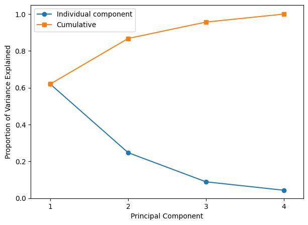
In this case, if we want to preserve at least 80% of variance of the data, we need to select 2 PCs.
9.1.4. PCA on toy data and system transparency
Here, we adapt the example “Principal Component Regression vs Partial Least Squares Regression” from scikit-learn to explain the system transparency of PCA.
We generate synthetic data, perform PCA, and then plot the first two principal components:
rng = np.random.RandomState(0)
n_samples = 500
cov = [[3, 3], [3, 4]]
X = rng.multivariate_normal(mean=[0, 0], cov=cov, size=n_samples)
pca = PCA(n_components=2).fit(X)

fig = plt.figure(figsize=(5, 8))

plt.scatter(X[:, 0], X[:, 1], alpha=0.3, label="samples")

for i, (comp, var) in enumerate(zip(pca.components_, pca.explained_variance_)):
    # comp = comp * var  # scale component by its variance explanation power
    plt.arrow(
        x=0,
        y=0,
        dx=comp[0],
        dy=comp[1],
        color=f"C{i + 1}",
        width=0.1,
        label=f"Principal component {i+1}",
        head_width=0.3,
    )

plt.arrow(
    x=0,
    y=0,
    dx=X[1, 0] * 0.85,
    dy=X[1, 1] * 0.85,
    color="k",
    width=0.1,
    head_width=0.3,
    label="Input Data Sample",
)
plt.scatter(
    X[1, 0],
    X[1, 1],
    alpha=0.8,
    facecolors="none",
    marker="o",
    edgecolors="r",
    linewidths=3,
)

plt.gca().set(
    aspect="equal",
    title="2-dimensional dataset with principal components",
    xlabel="first feature",
    ylabel="second feature",
)
plt.legend()
plt.show()
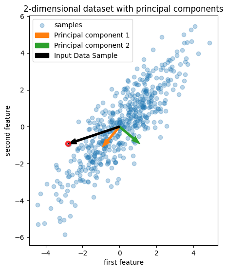
Let us examine the numerical values of a particular data point (circled in red), its principal component scores, the mean of the training data, the principal component loading vectors, and their explained variance.
print("The numbers display below round off to 2 decimal places.")
print("Data point: ", np.around(X[1, :], 2))
print(
    "Scores of the data point: ", np.around(pca.transform(X[1, :].reshape(1, -1))[0], 2)
)
print("Mean of the training data: ", np.around(pca.mean_, 2))
print("PCA loadings: \n", np.around(pca.components_, 2))
print("Explained variance: ", np.around(pca.explained_variance_, 2))
print("Explained variance ratio: ", np.around(pca.explained_variance_ratio_, 2))
The numbers display below round off to 2 decimal places.
Data point:  [-2.78 -0.93]
Scores of the data point:  [ 2.67 -1.54]
Mean of the training data:  [0.12 0.12]
PCA loadings:
 [[-0.64 -0.77]
 [ 0.77 -0.64]]
Explained variance:  [6.21 0.46]
Explained variance ratio:  [0.93 0.07]
System transparency
For data point \( [-2.78 \;\; -0.93]^{\top} \), the score vector of PCA can be obtained by
The above process can be used inversely to obtain the input data from the scores by times the transpose (i.e. the inverse due to orthonormality) of the loading matrix (\(\left[\begin{matrix} -0.64 & -0.77 \\ 0.77 & -0.64 \end{matrix}\right]^{\top}\)) on both sides and move the mean to the other side:
The reconstruction can also be interpreted from the geometric perspective. As displayed in the figure above, the input data point \( [-2.78 \;\; -0.93]^{\top} \) (the black vector) can be viewed as the linear combination of the two loading vectors (PC 1 and PC 2 in orange and green, respectively). The scores of the input data point are the coefficients of the linear combination. The reconstructed input data point is the linear combination of the scores and the loading vectors:
Thus, given any point in the output PCA space, we can reconstruct the input data point by the above process.
Note: numbers are limited to two decimal places for the sake of clarity.
9.1.5. Exercises
1. Load the mice protein dataset from sklearn.datasets using fetch_openml where the dataset contains gene expressions of mice brains and show the first 5 rows of the data. Hint: See here for further help.
# Write your code below to answer the question
Compare your answer with the reference solution below
from sklearn.datasets import fetch_openml

mnist = fetch_openml("miceprotein")
df = mnist.data.dropna()
df.head()
/opt/hostedtoolcache/Python/3.8.18/x64/lib/python3.8/site-packages/sklearn/datasets/_openml.py:1022: FutureWarning: The default value of `parser` will change from `'liac-arff'` to `'auto'` in 1.4. You can set `parser='auto'` to silence this warning. Therefore, an `ImportError` will be raised from 1.4 if the dataset is dense and pandas is not installed. Note that the pandas parser may return different data types. See the Notes Section in fetch_openml's API doc for details.
  warn(
| DYRK1A_N | ITSN1_N | BDNF_N | NR1_N | NR2A_N | pAKT_N | pBRAF_N | pCAMKII_N | pCREB_N | pELK_N | ... | SHH_N | BAD_N | BCL2_N | pS6_N | pCFOS_N | SYP_N | H3AcK18_N | EGR1_N | H3MeK4_N | CaNA_N | |
|---|---|---|---|---|---|---|---|---|---|---|---|---|---|---|---|---|---|---|---|---|---|
| 75 | 0.649781 | 0.828696 | 0.405862 | 2.921435 | 5.167979 | 0.207174 | 0.176640 | 3.728084 | 0.239283 | 1.666579 | ... | 0.239752 | 0.139052 | 0.112926 | 0.132001 | 0.129363 | 0.486912 | 0.125152 | 0.146865 | 0.143517 | 1.627181 |
| 76 | 0.616481 | 0.841974 | 0.388584 | 2.862575 | 5.194163 | 0.223433 | 0.167725 | 3.648240 | 0.221030 | 1.565150 | ... | 0.249031 | 0.133787 | 0.121607 | 0.139008 | 0.143084 | 0.467833 | 0.112857 | 0.161132 | 0.145719 | 1.562096 |
| 77 | 0.637424 | 0.852882 | 0.400561 | 2.968155 | 5.350820 | 0.208790 | 0.173261 | 3.814545 | 0.222300 | 1.741732 | ... | 0.247956 | 0.142324 | 0.130261 | 0.134804 | 0.147673 | 0.462501 | 0.116433 | 0.160594 | 0.142879 | 1.571868 |
| 78 | 0.576815 | 0.755390 | 0.348346 | 2.624901 | 4.727509 | 0.205892 | 0.161192 | 3.778530 | 0.194153 | 1.505475 | ... | 0.233225 | 0.133637 | 0.107321 | 0.118982 | 0.121290 | 0.479110 | 0.102831 | 0.144238 | 0.141681 | 1.646608 |
| 79 | 0.542545 | 0.757917 | 0.350051 | 2.634509 | 4.735602 | 0.210526 | 0.165671 | 3.871971 | 0.194297 | 1.531613 | ... | 0.244469 | 0.133358 | 0.112851 | 0.128635 | 0.142617 | 0.438354 | 0.110614 | 0.155667 | 0.146408 | 1.607631 |
5 rows × 77 columns
2. Using StandardScaler, standardise the loaded mice protein dataset from Exercise 1.
# Write your code below to answer the question
Compare your answer with the reference solution below
from sklearn.preprocessing import StandardScaler

scaler = StandardScaler()

X = scaler.fit_transform(df)
3. Now, run PCA from sklearn explaining at least \(95\%\) variance on the standardised mice protein dataset and display the top ten eigenvalues. Hint: Each eigenvalue represents the captured/explained variance in the direction of the respective eigenvector.
# Write your code below to answer the question
Compare your answer with the reference solution below
from sklearn.decomposition import PCA

pca = PCA(n_components=0.95)
pca.fit(X)

print(
    "The first 10 explained variance/eigenvalues are: \n", pca.explained_variance_[:10]
)
The first 10 explained variance/eigenvalues are:
 [23.09059993 13.38297469  7.60022832  7.17453775  3.28837408  3.04786113
  2.37162182  2.25936806  1.83407714  1.28103912]
4. Using the fitted PCA model in Exercise 3, find out the explained variance ratio for the top 10 principal components.
# Write your code below to answer the question
Compare your answer with the reference solution below
print(
    "The first 10 explained variance ratio are: \n", pca.explained_variance_ratio_[:10]
)
The first 10 explained variance ratio are:
 [0.29933466 0.17349    0.09852545 0.09300702 0.04262879 0.0395109
 0.03074449 0.02928929 0.02377603 0.01660673]
5. After observing the explained variance ratio from Exercise 4 carefully, find out how many principal components should we take to preserve \(70\%\) of variance of the data?
The first 5 principal components.
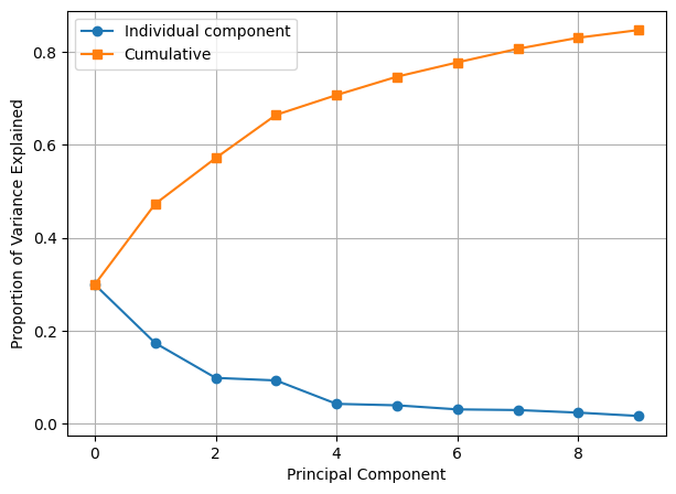
6. Finally, using the top 10 principal components, plot the PVE of each principal component and the cumulative PVE.
# Write your code below to answer the question
Compare your answer with the reference solution below
plt.figure(figsize=(7, 5))

plt.plot(pca.explained_variance_ratio_[:10], "-o", label="Individual component")
plt.plot(np.cumsum(pca.explained_variance_ratio_[:10]), "-s", label="Cumulative")

plt.ylabel("Proportion of Variance Explained")
plt.xlabel("Principal Component")

plt.legend(loc=2)
plt.grid()
plt.show()