Recurrent neural networks
Contents
10.3. Recurrent neural networks
Recurrent neural networks (RNNs) are a class of neural networks where connections between nodes (units/neurons) can create a directed cycle so that output from some nodes can affect subsequent input to the same node. RNNs are able to maintain an internal state that captures information about the sequence seen so far and they are able to use this internal state to make predictions about the next element in the sequence. This internal state is updated based on the input at each time step, and is used to make predictions about the next element in the sequence. RNNs are commonly used for processing sequential data such as text in natural language processing (NLP), speech in speech recognition, and time series in time series (e.g. stock price, weather) forecasting.
Watch the 15-minute video below for a visual explanation of recurrent neural networks.
Video
Explaining main ideas behind recurrent neural networks by StatQuest, embedded according to YouTube’s Terms of Service.
Remove or comment off the following installation if you have installed PyTorch and TorchVision already.
!pip3 install -q torch torchvision
[notice] A new release of pip is available: 23.0.1 -> 24.0
[notice] To update, run: pip install --upgrade pip
10.3.1. Why recurrent neural networks?
In the previous section, we saw how to use convolutional neural networks (CNNs) to process images. CNNs are a type of neural network that is particularly well suited to processing data that has a grid-like structure, such as images.
In this section, we will see how to use recurrent neural networks (RNNs) to process sequential data. RNNs are a type of neural network that is particularly well suited to processing data that has a temporal structure, such as text. In particular, they are able to maintain an internal state that captures information about the sequence seen so far. They can process sequences of variable length, unlike CNNs which can only process fixed-size inputs.
There are two key ideas behind RNNs:
Recurrent connections. RNNs have recurrent connections that allow information to flow through the network in a directed cycle. This allows the network to use its internal state to make predictions about the next element in the sequence.
Weight sharing. RNNs share weights across time steps. This means that the same weights are used to process the first element of the sequence, the second element, the third element, and so on. This allows the network to efficiently represent patterns that are consistent across time steps.
10.3.2. Unfolding a recurrent neural network
Fig. 10.5 shows a recurrent neural network in the compressed form on the left and the unfolded form for three time steps on the right. At each time step, the network takes an input and produces an output and a hidden state. The hidden state is then fed into the network at the next time step via the recurrent connection (labelled with ‘V’), e.g. from the hidden unit at time step \(t-1\) to the hidden unit at time step \(t\), and from the hidden unit at time step \(t\) to the hidden unit at time step \(t+1\). Note the weights and biases are shared across time steps.

Fig. 10.5 Unfolding a recurrent neural network across time steps
Let us see how RNNs work by going through an example adapted from the PyTorch tutorial Classifying Names with a Character-Level RNN with some modifications.
10.3.3. Get the data for surname classification
A character-level RNN reads words as a series of characters and outputs a prediction and “hidden state” at each step, feeding its previous hidden state into each next step. We take the final prediction to be the output, i.e. which class the word belongs to.
Specifically, we will train on a few thousand surnames from 18 languages of origin, and predict which language a name is from based on the spelling.
Get ready by importing the APIs needed from respective libraries and setting the random seed for reproducibility.
from __future__ import unicode_literals, print_function, division
from io import open
import glob
import os
import unicodedata
import string
import random
import time
import math

import torch
import torch.nn as nn
from torchvision.datasets.utils import download_and_extract_archive

import matplotlib.pyplot as plt
import matplotlib.ticker as ticker

torch.manual_seed(2022)
random.seed(2022)
Download and extract the data.
root_dir = "./data/"
data_url = "https://download.pytorch.org/tutorial/data.zip"
download_and_extract_archive(data_url, root_dir)
Downloading https://download.pytorch.org/tutorial/data.zip to ./data/data.zip
0%| | 0/2882130 [00:00<?, ?it/s]
100%|██████████| 2882130/2882130 [00:00<00:00, 127107190.87it/s]
Extracting ./data/data.zip to ./data/
Under the data/names directory, there are 18 text files named as “[Language].txt”. Each file contains a bunch of names, one name per line, mostly romanized but we still need to convert from Unicode to ASCII.
Let us examine the extracted files.
def findFiles(path):
    return glob.glob(path)


print(findFiles(root_dir + "data/names/*.txt"))
['./data/data/names/French.txt', './data/data/names/Greek.txt', './data/data/names/Chinese.txt', './data/data/names/Dutch.txt', './data/data/names/Russian.txt', './data/data/names/Arabic.txt', './data/data/names/Japanese.txt', './data/data/names/Spanish.txt', './data/data/names/Korean.txt', './data/data/names/Vietnamese.txt', './data/data/names/Italian.txt', './data/data/names/Portuguese.txt', './data/data/names/Czech.txt', './data/data/names/Scottish.txt', './data/data/names/German.txt', './data/data/names/Polish.txt', './data/data/names/English.txt', './data/data/names/Irish.txt']
10.3.4. Preprocess text data
10.3.4.1. Build a dictionary for names
Turn a Unicode string to plain ASCII based on a Stack Overflow post.
all_letters = string.ascii_letters + " .,;'"
n_letters = len(all_letters)


def unicodeToAscii(s):
    return "".join(
        c
        for c in unicodedata.normalize("NFD", s)
        if unicodedata.category(c) != "Mn" and c in all_letters
    )


print(unicodeToAscii("Ślusàrski"))
Slusarski
Build the category_lines dictionary, which contains a list of names per language {language: [names ...]}, by reading the files and splitting into lines.
category_lines = {}
all_categories = []


# Read a file and split into lines
def readLines(filename):
    lines = open(filename, encoding="utf-8").read().strip().split("\n")
    return [unicodeToAscii(line) for line in lines]


for filename in findFiles(root_dir + "data/names/*.txt"):
    category = os.path.splitext(os.path.basename(filename))[0]
    all_categories.append(category)
    lines = readLines(filename)
    category_lines[category] = lines

n_categories = len(all_categories)
Let us examine the dictionary by printing a few names for Italian.
print(category_lines["Italian"][:5])
['Abandonato', 'Abatangelo', 'Abatantuono', 'Abate', 'Abategiovanni']
10.3.4.2. Code names into tensors using one-hot encoding
Next, we need to represent each letter in a name by a one-hot vector. To represent a single letter, we use a “one-hot vector” of size <1 x n_letters>. A one-hot vector is filled with 0s except for a 1 at index of the current letter, e.g. "b" = <0 1 0 0 0 ...>.
To make a word we join a bunch of those into a 2D matrix <line_length x 1 x n_letters>. That extra 1 dimension is because PyTorch assumes everything is in batches - we’re just using a batch size of 1 here.
# Find the letter index from all_letters, e.g. "a" = 0
def letterToIndex(letter):
    return all_letters.find(letter)


# Turn a letter into a <1 x n_letters> tensor
def letterToTensor(letter):
    tensor = torch.zeros(1, n_letters)
    tensor[0][letterToIndex(letter)] = 1
    return tensor


# Turn a line into a <line_length x 1 x n_letters> tensor
def lineToTensor(line):
    tensor = torch.zeros(len(line), 1, n_letters)
    for li, letter in enumerate(line):
        tensor[li][0][letterToIndex(letter)] = 1
    return tensor


print(letterToTensor("J"))
print(lineToTensor("Jones").size())
tensor([[0., 0., 0., 0., 0., 0., 0., 0., 0., 0., 0., 0., 0., 0., 0., 0., 0., 0.,
         0., 0., 0., 0., 0., 0., 0., 0., 0., 0., 0., 0., 0., 0., 0., 0., 0., 1.,
         0., 0., 0., 0., 0., 0., 0., 0., 0., 0., 0., 0., 0., 0., 0., 0., 0., 0.,
         0., 0., 0.]])
torch.Size([5, 1, 57])
The following is how a single name is represented as a tensor.
print(lineToTensor("Jones"))
tensor([[[0., 0., 0., 0., 0., 0., 0., 0., 0., 0., 0., 0., 0., 0., 0., 0., 0.,
          0., 0., 0., 0., 0., 0., 0., 0., 0., 0., 0., 0., 0., 0., 0., 0., 0.,
          0., 1., 0., 0., 0., 0., 0., 0., 0., 0., 0., 0., 0., 0., 0., 0., 0.,
          0., 0., 0., 0., 0., 0.]],

        [[0., 0., 0., 0., 0., 0., 0., 0., 0., 0., 0., 0., 0., 0., 1., 0., 0.,
          0., 0., 0., 0., 0., 0., 0., 0., 0., 0., 0., 0., 0., 0., 0., 0., 0.,
          0., 0., 0., 0., 0., 0., 0., 0., 0., 0., 0., 0., 0., 0., 0., 0., 0.,
          0., 0., 0., 0., 0., 0.]],

        [[0., 0., 0., 0., 0., 0., 0., 0., 0., 0., 0., 0., 0., 1., 0., 0., 0.,
          0., 0., 0., 0., 0., 0., 0., 0., 0., 0., 0., 0., 0., 0., 0., 0., 0.,
          0., 0., 0., 0., 0., 0., 0., 0., 0., 0., 0., 0., 0., 0., 0., 0., 0.,
          0., 0., 0., 0., 0., 0.]],

        [[0., 0., 0., 0., 1., 0., 0., 0., 0., 0., 0., 0., 0., 0., 0., 0., 0.,
          0., 0., 0., 0., 0., 0., 0., 0., 0., 0., 0., 0., 0., 0., 0., 0., 0.,
          0., 0., 0., 0., 0., 0., 0., 0., 0., 0., 0., 0., 0., 0., 0., 0., 0.,
          0., 0., 0., 0., 0., 0.]],

        [[0., 0., 0., 0., 0., 0., 0., 0., 0., 0., 0., 0., 0., 0., 0., 0., 0.,
          0., 1., 0., 0., 0., 0., 0., 0., 0., 0., 0., 0., 0., 0., 0., 0., 0.,
          0., 0., 0., 0., 0., 0., 0., 0., 0., 0., 0., 0., 0., 0., 0., 0., 0.,
          0., 0., 0., 0., 0., 0.]]])
10.3.5. Define a recurrent neural network
We can implement a simple recurrent neural network (RNN) in PyTorch using regular feed-forward layers below, with two linear (fully-connected) layers operating on an input and hidden state and a LogSoftmax layer before the final output.
class RNN(nn.Module):
    def __init__(self, input_size, hidden_size, output_size):
        super(RNN, self).__init__()

        self.hidden_size = hidden_size

        self.i2h = nn.Linear(input_size + hidden_size, hidden_size)  # input to hidden
        self.i2o = nn.Linear(input_size + hidden_size, output_size)  # input to output
        self.softmax = nn.LogSoftmax(dim=1)

    def forward(self, input, hidden):
        combined = torch.cat((input, hidden), 1)
        hidden = self.i2h(combined)
        output = self.i2o(combined)
        output = self.softmax(output)
        return output, hidden

    def initHidden(self):
        return torch.zeros(1, self.hidden_size)


n_hidden = 128
rnn = RNN(n_letters, n_hidden, n_categories)
This RNN is illustrated in Fig. 10.6 below.

Fig. 10.6 A recurrent neural network module with two linear (fully-connected) layers.
To run a step of this RNN, we need to provide an input (the tensor for the current letter in this example) and a previous hidden state (with initialisation to zeros). At each step, we get the output as the probability of each language and a next hidden state for the next step.
input = letterToTensor("A")
hidden = torch.zeros(1, n_hidden)

output, next_hidden = rnn(input, hidden)
For efficiency, we will not create a new tensor for every step. Instead, we will use lineToTensor rather than letterToTensor and then operate on slices of lineTensor.
input = lineToTensor("Albert")
hidden = torch.zeros(1, n_hidden)

output, next_hidden = rnn(input[0], hidden)
print(output)
tensor([[-2.8592, -2.8253, -2.8707, -2.8112, -2.9611, -2.9083, -2.9330, -2.9325,
         -2.9786, -2.9515, -2.8053, -2.8357, -2.9486, -2.9308, -2.8328, -2.8497,
         -2.9542, -2.8667]], grad_fn=<LogSoftmaxBackward0>)
Here, the output is a <1 x 18> tensor (n_categories=18), where every item is the likelihood of that category (higher is more likely).
10.3.6. Optimisation, training and testing
10.3.6.1. Prepare for training
Before training, we make a few helper functions ready. The first is to interpret the output of the network, which we know to be a likelihood of each category. We can use Tensor.topk to get the index of the greatest value:
def categoryFromOutput(output):
    top_n, top_i = output.topk(1)
    category_i = top_i[0].item()
    return all_categories[category_i], category_i


print(categoryFromOutput(output))
('Italian', 10)
We also need a quick way to get a training example (a name and its language) randomly. We show 10 such random examples.
def randomChoice(list):
    return list[random.randint(0, len(list) - 1)]


def randomTrainingExample():
    category = randomChoice(all_categories)
    line = randomChoice(category_lines[category])
    category_tensor = torch.tensor([all_categories.index(category)], dtype=torch.long)
    line_tensor = lineToTensor(line)
    return category, line, category_tensor, line_tensor


for i in range(10):
    category, line, category_tensor, line_tensor = randomTrainingExample()
    print("category =", category, "/ line =", line)
category = Irish / line = Fionn
category = German / line = Schultheiss
category = Vietnamese / line = Vu
category = English / line = Thonon
category = Scottish / line = Shaw
category = Italian / line = Abbatelli
category = Scottish / line = Mackenzie
category = German / line = Schulz
category = English / line = Mustafa
category = Greek / line = Tsahalis
10.3.6.2. Choose a criterion and an optimiser
We choose the loss function nn.NLLLoss since the last layer of the RNN is nn.LogSoftmax.
learning_rate = 0.005  # A higher value may explode and a lower value may not learn.

criterion = nn.NLLLoss()
optimizer = torch.optim.SGD(rnn.parameters(), lr=learning_rate)
10.3.6.3. Train the network
Now, we are ready to train this RNN by showing it a bunch of examples, having it make predictions, and computing the loss for gradient descent.
Each loop of training will:
Create input and target tensors
Create a zeroed initial hidden state
Read each letter in and keep hidden state for next letter
Compare final output to target
Backpropagate
Return the output and loss
def train(category_tensor, line_tensor):
    hidden = rnn.initHidden()

    optimizer.zero_grad()  # Clear the gradients

    for i in range(line_tensor.size()[0]):
        output, hidden = rnn(line_tensor[i], hidden)

    loss = criterion(output, category_tensor)
    loss.backward()
    optimizer.step()

    return output, loss.item()
Now, we run this RNN with a bunch of examples. Since the train function returns both the output and loss we can print its predictions and keep track of loss for plotting. Since there are 1000s of examples, we print only every print_every examples and take an average of the loss.
n_iters = 60000
print_every = 2000
plot_every = 500

# Keep track of losses for plotting
current_loss = 0
all_losses = []


def timeSince(since):
    now = time.time()
    s = now - since
    m = math.floor(s / 60)
    s -= m * 60
    return "%dm %ds" % (m, s)


start = time.time()

for iter in range(1, n_iters + 1):
    category, line, category_tensor, line_tensor = randomTrainingExample()
    output, loss = train(category_tensor, line_tensor)
    current_loss += loss

    # Print iter number, loss, name and prediction
    if iter % print_every == 0:
        predicted, predicted_i = categoryFromOutput(output)
        correct = "✓" if predicted == category else "✗ (%s)" % category
        print(
            "%d %d%% (%s) %.4f %s / %s %s"
            % (
                iter,
                iter / n_iters * 100,
                timeSince(start),
                loss,
                line,
                predicted,
                correct,
            )
        )

    # Add current loss avg to list of losses
    if iter % plot_every == 0:
        all_losses.append(current_loss / plot_every)
        current_loss = 0
2000 3% (0m 1s) 2.8034 Chu / Vietnamese ✗ (Korean)
4000 6% (0m 3s) 2.5998 Sekigawa / Japanese ✓
6000 10% (0m 5s) 2.0556 Imendaev / Russian ✓
8000 13% (0m 7s) 1.6407 Zha / Korean ✗ (Chinese)
10000 16% (0m 9s) 2.1380 Marquerink / Czech ✗ (Dutch)
12000 20% (0m 11s) 1.3932 Jbanov / Russian ✓
14000 23% (0m 12s) 2.5772 Brant / Vietnamese ✗ (German)
16000 26% (0m 14s) 1.8472 Petrezelka / Greek ✗ (Czech)
18000 30% (0m 16s) 2.0134 Frampton / Russian ✗ (English)
20000 33% (0m 18s) 0.7730 Yue / Chinese ✓
22000 36% (0m 20s) 1.3608 Saksagansky / Polish ✗ (Russian)
24000 40% (0m 22s) 2.6653 Rossum / Arabic ✗ (Dutch)
26000 43% (0m 24s) 0.4203 Chrysanthopoulos / Greek ✓
28000 46% (0m 25s) 1.3604 Fonseca / Spanish ✓
30000 50% (0m 27s) 0.5601 Orsini / Italian ✓
32000 53% (0m 29s) 0.4405 Than / Vietnamese ✓
34000 56% (0m 31s) 1.2924 Bhrighde / Irish ✓
36000 60% (0m 33s) 1.3770 Overton / English ✓
38000 63% (0m 35s) 1.5098 Wasem / Arabic ✓
40000 66% (0m 37s) 3.5593 Niftrik / Czech ✗ (Dutch)
42000 70% (0m 38s) 0.5813 Chu / Vietnamese ✓
44000 73% (0m 40s) 0.0886 Winogrodzki / Polish ✓
46000 76% (0m 42s) 1.2651 Gwang / Korean ✓
48000 80% (0m 44s) 0.2295 Handal / Arabic ✓
50000 83% (0m 46s) 2.1338 Svoboda / Spanish ✗ (Czech)
52000 86% (0m 48s) 0.5378 Arakida / Japanese ✓
54000 90% (0m 49s) 0.7451 Kramer / German ✓
56000 93% (0m 51s) 0.3432 Byon / Korean ✓
58000 96% (0m 53s) 0.1131 Bukowski / Polish ✓
60000 100% (0m 55s) 0.9363 Maroun / Arabic ✓
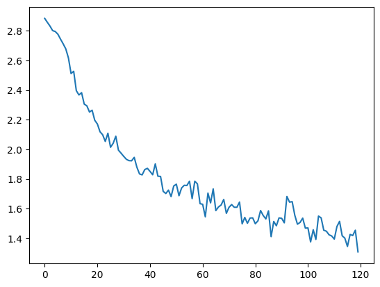
10.3.6.4. Plot the loss
Plotting the historical loss from all_losses shows how the network learned over time.
plt.figure()
plt.plot(all_losses)
[<matplotlib.lines.Line2D at 0x7faf6d4fe280>]
10.3.6.5. Evaluate the results
To see how well the network performs on different categories, we will create a confusion matrix, indicating for every actual language (rows) which language the network has predicted to be (columns). To calculate the confusion matrix, a bunch of samples are run through the network with evaluate(), which is the same as train() minus the backprop.
# Keep track of correct predictions in a confusion matrix
confusion = torch.zeros(n_categories, n_categories)
n_confusion = 10000


# Just return an output given a line
def evaluate(line_tensor):
    hidden = rnn.initHidden()

    for i in range(line_tensor.size()[0]):
        output, hidden = rnn(line_tensor[i], hidden)

    return output


# Go through a bunch of examples and record which are correctly predicted
for i in range(n_confusion):
    category, line, category_tensor, line_tensor = randomTrainingExample()
    output = evaluate(line_tensor)
    predicted, predicted_i = categoryFromOutput(output)
    category_i = all_categories.index(category)
    confusion[category_i][predicted_i] += 1

# Normalize by dividing every row by its sum
for i in range(n_categories):
    confusion[i] = confusion[i] / confusion[i].sum()

# Set up plot
fig = plt.figure()
ax = fig.add_subplot(111)
cax = ax.matshow(confusion.numpy())
fig.colorbar(cax)

# Set up axes
ax.set_xticklabels([""] + all_categories, rotation=90)
ax.set_yticklabels([""] + all_categories)

# Force label at every tick
ax.xaxis.set_major_locator(ticker.MultipleLocator(1))
ax.yaxis.set_major_locator(ticker.MultipleLocator(1))

plt.show()
/tmp/ipykernel_2859/1638848402.py:35: UserWarning: FixedFormatter should only be used together with FixedLocator
  ax.set_xticklabels([""] + all_categories, rotation=90)
/tmp/ipykernel_2859/1638848402.py:36: UserWarning: FixedFormatter should only be used together with FixedLocator
  ax.set_yticklabels([""] + all_categories)
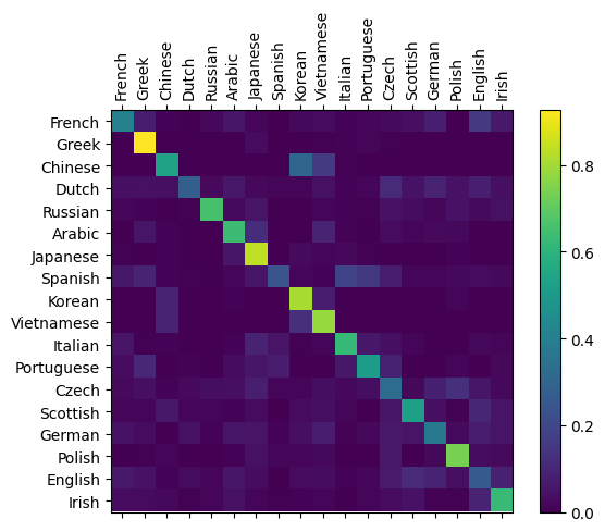
We can pick out bright spots off the main axis that show which languages it has most confusion with, e.g. Chinese for Korean. It seems to do very well with Greek, and very poorly with English (perhaps because of overlap with other languages).
10.3.6.6. Test on user input
We can also run the network on user input to see what it predicts.
def predict(input_line, n_predictions=3):
    print("\n> %s" % input_line)
    with torch.no_grad():
        output = evaluate(lineToTensor(input_line))

        # Get top N categories
        topv, topi = output.topk(n_predictions, 1, True)
        predictions = []

        for i in range(n_predictions):
            value = topv[0][i].item()
            category_index = topi[0][i].item()
            print("(%.2f) %s" % (value, all_categories[category_index]))
            predictions.append([value, all_categories[category_index]])


predict("Hinton")
predict("Schmidhuber")
predict("Zhou")
> Hinton
(-1.01) Scottish
(-1.58) English
(-2.27) Russian

> Schmidhuber
(-1.48) Russian
(-1.83) Polish
(-1.90) Arabic

> Zhou
(-0.50) Korean
(-1.55) Chinese
(-2.21) Vietnamese
Do these predictions make sense to you?
10.3.7. Advanced RNNs
There are more advanced RNNs that can be used for sequence modelling, such as the Long Short-Term Memory (LSTM), Gated Recurrent Unit (GRU), and Transformer. These networks are more complex and are beyond the scope of this course. However, you can find more information about them in the PyTorch documentation.
10.3.8. Exercises
1. How is a recurrent neural network different from a convolutional neural network?
Compare your answer with the solution below
CNNs are a type of neural networks that is particularly well suited to processing data that has a grid-like structure, such as images, whereas RNNs are particularly well suited to processing data that has a sequence structure, such as text.
2. What are the two key ideas behind RNNs?
Compare your answer with the solution below
The two key ideas behind RNNs are recurrent connections and weight sharing.
3. What is the purpose of recurrent connections in RNNs?
Compare your answer with the solution below
Recurrent connections allow information to flow through the network in a directed cycle, allowing the network to use its internal state to make predictions about the next element in the sequence.
4. What is the purpose of weight sharing in RNNs?
Compare your answer with the solution below
Weight sharing in RNNs means that the same weights are used to process all time steps, which allows the network to efficiently represent patterns that are consistent across steps.