Logistic regression
Contents
3.2. Logistic regression
Although having “regression” in its name, logistic regression is a classification (rather than regression) algorithm. Instead of modelling the qualitative response \(y\) directly, logistic regression models the probability that \(y\) belongs to a particular class (category).
Watch the 8-minute video below for a visual explanation of logistic regression:
Video
Explaining Logistic Regression by StatQuest, embedded according to YouTube’s Terms of Service.
3.2.1. Import libraries and load data
Get ready by importing the APIs needed from respective libraries.
import pandas as pd
import numpy as np
from matplotlib.gridspec import GridSpec
import matplotlib.pyplot as plt
import seaborn as sns

from sklearn.linear_model import LogisticRegression
from sklearn.metrics import accuracy_score, roc_auc_score, RocCurveDisplay

from statsmodels.formula.api import logit

%matplotlib inline
Load the Default dataset and inspect the first three rows.
data_url = "https://github.com/pykale/transparentML/raw/main/data/Default.csv"
df = pd.read_csv(data_url)

# Note: factorize() returns two objects: a label array and an array with the unique values. We are only interested in the first object.
df["default2"] = df.default.factorize()[0]
df["student2"] = df.student.factorize()[0]
df.head(3)
| default | student | balance | income | default2 | student2 | |
|---|---|---|---|---|---|---|
| 0 | No | No | 729.526495 | 44361.625074 | 0 | 0 |
| 1 | No | Yes | 817.180407 | 12106.134700 | 0 | 1 |
| 2 | No | No | 1073.549164 | 31767.138947 | 0 | 0 |
3.2.2. Logistic model
Logistic regression models the probability that the response \(y\) belongs to a particular class (category) using linear regression via a logistic function, hence the name logistic regression. For binary classification, let us use 1 to denote the positive class (e.g. “Yes”) and 0 to denote the negative class (e.g. “No”).
3.2.2.1. Logit function transformation
Let \(\pi\) be the probability of a positive outcome
Then the probability of a negative outcome \( \mathbb{P}(y=0| x) = 1-\pi \).
The odds of a positive outcome is the ratio of the probability of a positive outcome to the probability of a negative outcome, i.e.
The log of the odds is called the logit and the logit function is defined as :
The logit function is a monotonic transformation of the probability \(\pi\). It maps the probability \(\pi\) ranging from 0 to 1 to the real line ranging from \(-\infty\) to \(\infty\). The logit function is also known as the log-odds function.
3.2.2.2. Logistic function
In simple linear regression, we have modelled the relationship between outcome \(y\) and feature \(x\) with a linear equation:
This linear regression model is not able to produce a binary outcome for binary classification or a probability (in the range from 0 to 1 only). With the logit function above, we can transform the probability \(\pi\) ranging from 0 to 1 to the logit function \(\mathrm{logit}(\pi)\) ranging from \(-\infty\) to \(\infty\). Now we can use the linear regression model to model the logit function \(\mathrm{logit}(\pi)\) instead of the probability \(\pi\) or \(y\) directly. The logit function is defined as:
The logistic function, also known as the sigmoid function, is the inverse of the logit function. It maps the logit function \(\mathrm{logit}(\pi)\) ranging from \(-\infty\) to \(\infty\) to the probability \(\pi\) ranging from 0 to 1:
3.2.3. Estimating the coefficients to make predictions
The coefficients of a logistic regression model can be estimated by maximum likelihood estimation (MLE). The likelihood function is
The mathematical details are beyond the scope of this course. If interested, please read Section 4.3 of the Pattern Recognition and Machine Learning book for more details of the optimization for logistic regression.
To make predictions, taking the classification problem on the Default dataset, the probability of default given balance predicted by a logistic regression model is
3.2.3.1. Example explanation of system transparency
Let us to see the curve of the logistic function on the Default dataset.
sns.regplot(data=df, x="balance", y="default2", logistic=True)
plt.ylabel("Probability of default")
plt.xlabel("Balance")
plt.show()
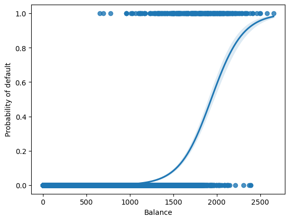
We can see an S-shaped curve with the vertical axis ranging from 0 to 1, indicating the probability of a positive outcome (default) with respect to the horizontal axis \(x\) (balance).
In practice, we can use the scikit-learn or statsmodels package to fit a logistic regression model and make predictions.
Let us fit a logistic regression model using the scikit-learn API for logistic regression first.
clf = LogisticRegression(solver="newton-cg")
X_train = df.balance.values.reshape(-1, 1)
X_test = np.arange(df.balance.min(), df.balance.max()).reshape(-1, 1)
y = df.default2
clf.fit(X_train, y)
print(clf)
print("classes: ", clf.classes_)
print("coefficients: ", clf.coef_)
print("intercept :", clf.intercept_)
LogisticRegression(solver='newton-cg')
classes:  [0 1]
coefficients:  [[0.00549892]]
intercept : [-10.65132978]
Let us plot the fitted logistic regression model and study the system transparency.
prob = clf.predict_proba(X_test)

plt.scatter(X_train, y, color="orange")
plt.plot(X_test, prob[:, 1], color="lightblue")

plt.hlines(
    1,
    xmin=plt.gca().xaxis.get_data_interval()[0],
    xmax=plt.gca().xaxis.get_data_interval()[1],
    linestyles="dashed",
    lw=1,
)
plt.hlines(
    0,
    xmin=plt.gca().xaxis.get_data_interval()[0],
    xmax=plt.gca().xaxis.get_data_interval()[1],
    linestyles="dashed",
    lw=1,
)

plt.hlines(
    0.5,
    xmin=plt.gca().xaxis.get_data_interval()[0],
    xmax=plt.gca().xaxis.get_data_interval()[1],
    linestyles="dashed",
    lw=1,
)

plt.vlines(
    -clf.intercept_ / clf.coef_[0],
    ymin=plt.gca().yaxis.get_data_interval()[0],
    ymax=plt.gca().yaxis.get_data_interval()[1],
    linestyles="dashed",
    lw=1,
)

plt.hlines(
    (clf.predict_proba(np.asarray(1500).reshape(-1, 1)))[0][1],
    xmin=plt.gca().xaxis.get_data_interval()[0],
    xmax=1500,
    linestyles="dashed",
    lw=1,
)

plt.vlines(
    1500,
    ymin=plt.gca().yaxis.get_data_interval()[0],
    ymax=(clf.predict_proba(np.asarray(1500).reshape(-1, 1)))[0][1],
    linestyles="dashed",
    lw=1,
)

plt.ylabel("Probability of default")
plt.xlabel("Balance")
plt.yticks([0, 0.25, 0.5, 0.75, 1.0])
plt.xlim(xmin=-100)
plt.show()
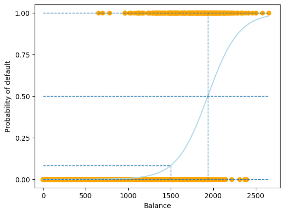
In the above example, we learnt a logistic regression model \(f(x)\) with two parameters, \(\beta_0\) and \(\beta_1\), from the data, where
\(\beta_0 = -10.65133019 \)
\(\beta_1 = 0.00549892 \)
Using these two estimated parameters, we can examine the system logic of the logistic regression model to reveal its system transparency.
System transparency
When
balance=1500 , the predicted probability ofdefaultis
When the probability of
default0.5 (the commonly used threshold for binary classification), the corresponding balance can be calculated using the log odds equation above:
Therefore, to produce result Yes, i.e. for the probability of default \(>\) 0.5, the balance should be greater than 1936.9858426745614. Likewise, to produce result No, i.e. the probability of default \(<\) 0.5, the balance should be less than 1936.9858426745614.
Let us fit a logistic regression model using the [statsmodels API for logistic regression] next.
est = logit("default2 ~ balance", df).fit()
est.summary2().tables[1]
Optimization terminated successfully.
         Current function value: 0.079823
         Iterations 10
| Coef. | Std.Err. | z | P>|z| | [0.025 | 0.975] | |
|---|---|---|---|---|---|---|
| Intercept | -10.651331 | 0.361169 | -29.491287 | 3.723665e-191 | -11.359208 | -9.943453 |
| balance | 0.005499 | 0.000220 | 24.952404 | 2.010855e-137 | 0.005067 | 0.005931 |
We can see that the estimated parameters are the same as those from the scikit-learn API. Note the two last columns, “[0.025” and “0.975]”. These are Confidence Intervals, the very concept we covered in the last chapter on Linear Regression! Now, let us fit a logistic regression model using student status as the input variable.
est = logit("default2 ~ student", df).fit()
est.summary2().tables[1]
Optimization terminated successfully.
         Current function value: 0.145434
         Iterations 7
| Coef. | Std.Err. | z | P>|z| | [0.025 | 0.975] | |
|---|---|---|---|---|---|---|
| Intercept | -3.504128 | 0.070713 | -49.554094 | 0.000000 | -3.642723 | -3.365532 |
| student[T.Yes] | 0.404887 | 0.115019 | 3.520177 | 0.000431 | 0.179454 | 0.630320 |
The coefficient associated with student is positive, indicating that the probability of default is higher for students than non-students.
3.2.4. Multiple logistic regression
The logistic regression model can be extended to multiple features. A generalised logistic regression model for an instance \(\mathbf{x} = [x_1, x_2, \dots, x_D]^\top\) is
Let us fit a multiple logistic regression model using the scikit-learn API first.
Let us plot the fitted multiple logistic regression model and study the system transparency.
import warnings

warnings.filterwarnings("ignore")

X_train = df.loc[:, ["balance", "income", "student2"]]
y = df.default2

clf = LogisticRegression(solver="newton-cg", penalty="none", max_iter=1000)
clf.fit(X_train, y)
print(clf)
print("classes: ", clf.classes_)
print("coefficients: ", clf.coef_)
print("intercept :", clf.intercept_)
LogisticRegression(max_iter=1000, penalty='none', solver='newton-cg')
classes:  [0 1]
coefficients:  [[ 5.73139387e-03  2.83615167e-06 -6.51143222e-01]]
intercept : [-10.85258456]
Let us fit a multiple logistic regression model using the statsmodels API next.
est = logit("default2 ~ balance + income + student", df).fit()
est.summary2().tables[1]
Optimization terminated successfully.
         Current function value: 0.078577
         Iterations 10
| Coef. | Std.Err. | z | P>|z| | [0.025 | 0.975] | |
|---|---|---|---|---|---|---|
| Intercept | -10.869045 | 0.492273 | -22.079320 | 4.995499e-108 | -11.833882 | -9.904209 |
| student[T.Yes] | -0.646776 | 0.236257 | -2.737595 | 6.189022e-03 | -1.109831 | -0.183721 |
| balance | 0.005737 | 0.000232 | 24.736506 | 4.331521e-135 | 0.005282 | 0.006191 |
| income | 0.000003 | 0.000008 | 0.369808 | 7.115254e-01 | -0.000013 | 0.000019 |
Similar parameters are estimated as using the scikit-learn API.
3.2.5. Evaluation of logistic regression
The evaluation of logistic regression is similar to the evaluation of linear regression. The main difference is that the evaluation metrics are different. For example, the mean squared error (MSE) is not a good metric for classification. Here we introduce two common metrics for classification: accuracy and area under receiver operating characteristic (ROC) curve, i.e. AUC (or more precisely, AUROC).
3.2.5.1. Accuracy
The accuracy is the fraction of correct predictions. It is defined as
Let us compute the training accuracy of the multiple logistic regression model trained using scikit-learn API above.
y_pred = clf.predict(X_train)
accuarcy = accuracy_score(y, y_pred)
print("Accuracy: ", accuarcy)
Accuracy: 0.9732
3.2.5.2. Area under the ROC curve (AUC)
The receiver operating characteristic (ROC) curve is a plot of the true positive rate (TPR) against the false positive rate (FPR) at various threshold settings. The TPR and FPR are defined as
The area under the ROC curve (AUC) is a popular measure of classifier performance. The AUC is defined as the area under the ROC curve. It is a number between 0 and 1, where 0.5 is the random guess and 1 is the perfect prediction. The AUC is a good metric for evaluating the classification since it considers all possible classification thresholds.
Let us plot the ROC curve of the multiple logistic regression model trained using scikit-learn API above.
y_prob = clf.predict_proba(X_train)[:, 1]

roc_auc = roc_auc_score(y, y_prob)
print("AUC: ", roc_auc)

clf_disp = RocCurveDisplay.from_estimator(clf, X_train, y)
plt.show()
AUC: 0.949552531739353
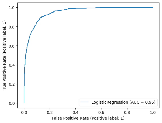
We can see clearly the trade-off between TPR and FPR. The AUC is 0.95, indicating that the model is good.
3.2.6. Exercise
1. Logistic regression is a classification algorithm.
    a. True

    b. False
Compare your answer with the solution below
a. True
2. All the following exercises will use the Weekly dataset.
Load the dataset, convert the categories to numerical values, and fit a logistic regression model using Volume variable as a predictor and Direction variable as the response using scikit-learn or statsmodel. Find out the fitted model’s weight and bias.
# Write your code below to answer the question
Compare your answer with the reference solution below
import pandas as pd
import numpy as np
from matplotlib.gridspec import GridSpec
import matplotlib.pyplot as plt
import seaborn as sns

from sklearn.linear_model import LogisticRegression


data_url = "https://github.com/pykale/transparentML/raw/main/data/Weekly.csv"
df = pd.read_csv(data_url)
df["Direction"] = df.Direction.factorize()[0]

clf = LogisticRegression(solver="newton-cg")
X_train = df.Volume.values.reshape(-1, 1)
y = df.Direction
clf.fit(X_train, y)
print("coefficients: ", clf.coef_)
print("intercept :", clf.intercept_)
coefficients:  [[-0.0213956]]
intercept : [0.25689958]
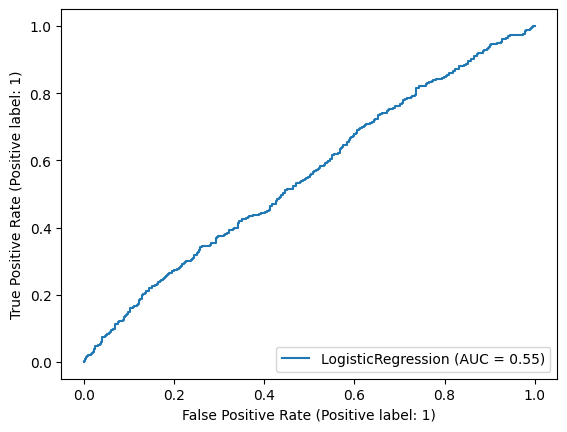
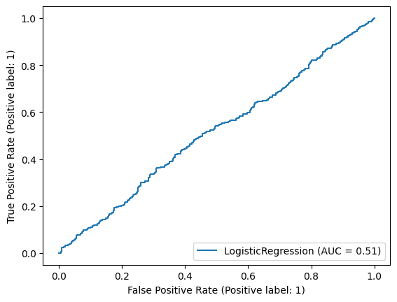
3. Plot the ROC curve and find out the training accuracy and AUC of the fitted model from Exercise 2.
# Write your code below to answer the question
Compare your answer with the reference solution below
from sklearn.metrics import accuracy_score, roc_auc_score, RocCurveDisplay

y_pred = clf.predict(X_train)
accuarcy = accuracy_score(y, y_pred)
print("Training Accuracy: ", accuarcy)

y_prob = clf.predict_proba(X_train)[:, 1]
roc_auc = roc_auc_score(y, y_prob)
print("AUC: ", roc_auc)

clf_disp = RocCurveDisplay.from_estimator(clf, X_train, y)
plt.show()

# From the ROC curve we can say that the result is almost random as it is almost close to 50%.
# The model from Exercise-2 has not learnt anything at all.
Training Accuracy:  0.5555555555555556
AUC:  0.5142783962844069
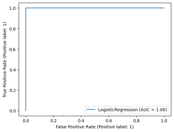
4. Train another logistic regression model using Direction as a response and all the other features as predictors. Print out all the parameter values.
# Write your code below to answer the question
Compare your answer with the reference solution below
X_train = df.drop(["Direction"], axis=1)

y = df.Direction

clf = LogisticRegression(solver="newton-cg")
clf.fit(X_train, y)
print("coefficients: ", clf.coef_)
print("intercept :", clf.intercept_)
coefficients:  [[ 3.68485224e-03 -8.79795063e-02  4.30643833e-02  1.39945670e-02
  -1.71842138e-02  6.21526979e-02  7.95815168e-02  7.22161831e+00]]
intercept : [-7.36769879]
5. Plot the ROC curve and find out the training accuracy and AUC metrics of the fitted model from Exercise 4.
# Write your code below to answer the question
Compare your answer with the reference solution below
y_pred = clf.predict(X_train)
accuarcy = accuracy_score(y, y_pred)
print("Training Accuracy: ", accuarcy)

y_prob = clf.predict_proba(X_train)[:, 1]
roc_auc = roc_auc_score(y, y_prob)
print("AUC: ", roc_auc)

clf_disp = RocCurveDisplay.from_estimator(clf, X_train, y)
plt.show()

# The model from Exercise 4 learnt very well on the training dataset.
Training Accuracy:  0.9972451790633609
AUC:  0.9999931698654464
6. You might notice that the model with all variables is much better than the model from Exercise 2. Use the skills you have learnt to perform further analysis on the data to explain why. Hint: Consider correlations (See section 2.2.4)
# Write your code below to answer the question
Compare your answer with the reference solution below
corr_matrix = df.corr()
print(corr_matrix)
# Here from the correlation result we can see that, "Today" has a 0.72 correlation with "Direction"
# which is the main reason for getting high performance

y = df.Direction

# model with out "Today"
X_train = df.drop(["Direction", "Today"], axis=1)
clf.fit(X_train, y)
clf_disp = RocCurveDisplay.from_estimator(clf, X_train, y)
# Without today feature the model performed very bad

# model with only "Today"
X_train = df["Today"].values.reshape(-1, 1)
clf.fit(X_train, y)
clf_disp = RocCurveDisplay.from_estimator(clf, X_train, y)
# with today feature the model performed very well
# from this experiment we analyzed the important of correlation between feature and target variable
               Year      Lag1      Lag2      Lag3      Lag4      Lag5  \
Year       1.000000 -0.032289 -0.033390 -0.030006 -0.031128 -0.030519
Lag1      -0.032289  1.000000 -0.074853  0.058636 -0.071274 -0.008183
Lag2      -0.033390 -0.074853  1.000000 -0.075721  0.058382 -0.072499
Lag3      -0.030006  0.058636 -0.075721  1.000000 -0.075396  0.060657
Lag4      -0.031128 -0.071274  0.058382 -0.075396  1.000000 -0.075675
Lag5      -0.030519 -0.008183 -0.072499  0.060657 -0.075675  1.000000
Volume     0.841942 -0.064951 -0.085513 -0.069288 -0.061075 -0.058517
Today     -0.032460 -0.075032  0.059167 -0.071244 -0.007826  0.011013
Direction -0.022200 -0.050004  0.072696 -0.022913 -0.020549 -0.018168

             Volume     Today  Direction
Year       0.841942 -0.032460  -0.022200
Lag1      -0.064951 -0.075032  -0.050004
Lag2      -0.085513  0.059167   0.072696
Lag3      -0.069288 -0.071244  -0.022913
Lag4      -0.061075 -0.007826  -0.020549
Lag5      -0.058517  0.011013  -0.018168
Volume     1.000000 -0.033078  -0.017995
Today     -0.033078  1.000000   0.720025
Direction -0.017995  0.720025   1.000000