Feature selection
Contents
6.1. Feature selection
Feature selection is the process of selecting a subset of relevant features (predictors, variables) for use in model construction. Feature selection methods are an important part of any data science workflow because they allow us to reduce the complexity of our models, making them easier to interpret, and more robust to the effects of collinearity.
We will study feature selection in the context of linear regression models. The same principles apply to other types of models such as classification and clustering models.
6.1.1. Best subset selection
Let us consider the problem of selecting the best subset of features (predictors) for the classical linear regression model covered in the previous chapter Linear Regression. To perform this best feature subset selection, we can fit a separate least squares regression for each possible combination of the \(D\) predictors. That is, we fit
all \(\left(\begin{array}{c} D \\ 1 \end{array}\right)=D\) models that contain exactly one predictor,
all \(\left(\begin{array}{c} D \\ 2 \end{array}\right)=D(D − 1)/2\) models that contain exactly two predictors, and
all \(\left(\begin{array}{c} D \\ d \end{array}\right)\) models that contain exactly \(d\) predictors, for \(d = 3, \cdots, D\).
We then look at all of the resulting models, with the goal of identifying the one that is best.
Algorithm 6.1 (Best subset selection)
Let \(\mathcal{M}_0\) denote the null model, which contains no predictors. This model simply predicts the sample mean for each observation.
For \(d = 1, 2, \cdots, D\):
Fit all \(\left(\begin{array}{c} D \\ d \end{array}\right)\) models that contain exactly \(d\) predictors, where \(D\) is the total number of predictors.
Choose the best among these \(\left(\begin{array}{c} D \\ d \end{array}\right)\) models, denoted \(\mathcal{M}_d\). Here best is defined using some criterion, such as \(\mathrm{R}^2\) for linear regression (or AUC for binary classification).
Select the single best model from \(\mathcal{M}_0\), \(\mathcal{M}_1\), \(\cdots\), \(\mathcal{M}_D\) using cross-validation.
As you can imagine, the best subset selection algorithm above is computationally very expensive. For example, if we have \(D = 100\) predictors, then we would have to fit \(2^{100} = 1.3 \times 10^{30}\) models! Thus, for computational reasons, best subset selection can only be applied to problems with a very small number of predictors, making it practically useless for most real-world applications.
Best subset selection may also suffer from statistical problems when \(D\) is large. The larger the search space, the higher the chance of finding models that look good on the training (known/seen) data, even though they might not have any predictive power on test (unknown/unseen) data. Thus, an enormous search space can lead to high variance of the coefficient estimates and overfitting, where the model performs well on the training data but poorly on the test data.
For both reasons above, stepwise methods, which explore a far more restricted set of models, are attractive alternatives to best subset selection.
6.1.2. Stepwise selection
There are two main types of stepwise methods: forward stepwise selection and backward stepwise selection. In forward stepwise selection, we begin with the null model that contains no predictors, and then consider adding predictors one at a time until all \(D\) predictors have been added. In backward stepwise selection, we begin with the full model that contains all \(D\) predictors, and then consider removing predictors one at a time until we are left with the null model that contains no predictors.
6.1.2.1. Forward stepwise selection
Forward stepwise selection is a computationally efficient alternative to best subset selection. While the best subset selection procedure considers all \(2^D\) possible models containing subsets of the \(D\) predictors, forward stepwise considers a much smaller set of models. Forward stepwise selection begins with a model containing no predictors, and then adds predictors to the model, one-at-a-time, until all of the predictors are in the model. In particular, at each step the predictor (feature, variable) that gives the greatest additional improvement to the fit is added to the model. This is called a greedy search because at each step we choose the best option available, without looking ahead.
Algorithm 6.2 (Forward stepwise selection)
Let \(\mathcal{M}_0\) denote the null model, which contains no predictors. This model simply predicts the sample mean for each observation.
For \(d = 1, 2, \ldots, D\):
Fit all \(D - d + 1\) models that contain all of the predictors in \(\mathcal{M}_{d-1}\) plus one additional predictor.
Choose the best among these \(D - d + 1\) models, denoted \(\mathcal{M}_d\). Here best is defined using some criterion such as \(\mathrm{R}^2\) for linear regression.
Select the single best model from \(\mathcal{M}_0\), \(\mathcal{M}_1\), \(\cdots\), \(\mathcal{M}_D\) using cross-validation.
Unlike best subset selection, which involved fitting \(2^D\) models, forward stepwise selection involves fitting one null model, along with \(D − d\) models in the \(d\)th iteration, for \(d = 0, \dots, D − 1\). This amounts to a total of \(1 + \sum_{d=0}^{D-1}(D-d) = 1 + D(D+1)/2\) models. This is a substantial difference: when \(D = 20\), best subset selection requires fitting 1,048,576 models, whereas forward stepwise selection requires fitting only 211 models.
Forward stepwise selection’s computational advantage over best subset selection is clear. Though forward stepwise tends to do well in practice, it is not guaranteed to find the best possible model out of all \(2^D\) models containing subsets of the \(D\) predictors. For example, suppose that in a given dataset with \(D\) = 3 predictors, the best possible one-predictor model contains \(x_1\), and the best possible two-predictor model instead contains \(x_2\) and \(x_3\). Then forward stepwise selection will fail to select the best possible two-predictor model, because \(\mathcal{M}_1\) will contain \(x_1\), so \(\mathcal{M}_2\) must also contain \(x_1\) together with one additional predictor. This is common for stepwise methods (and greedy algorithms in general), which are guaranteed to find only a local optimum, not a global optimum.
6.1.2.2. Backward stepwise selection
Backward stepwise selection is similar to forward stepwise selection, except that it begins with the full model that contains all \(D\) predictors, and then removes the least useful predictor, one-at-a-time, until the model contains no predictors.
Algorithm 6.3 (Backward stepwise selection)
Let \(\mathcal{M}_0\) denote the null model, which contains no predictors. This model simply predicts the sample mean for each observation.
For \(d = D, D-1, \cdots, 1\):
Consider all \(d\) models that contain all but one of the predictors in \(\mathcal{M}_{d}\), for a total of \(d-1\) predictors.
Choose the best among these \( d \) models, denoted \(\mathcal{M}_{d-1}\). Here best is defined using some criterion such as \(\mathrm{R}^2\) for linear regression.
Select the single best model from \(\mathcal{M}_0\), \(\mathcal{M}_1\), \(\cdots\), \(\mathcal{M}_D\) using cross-validation.
Like forward stepwise selection, the backward selection approach searches through only \(1 + D(D + 1)/2\) models, and so can be applied in settings where \(D\) is too large to apply best subset selection. Also like forward stepwise selection, backward stepwise selection is a greedy algorithm, and so is not guaranteed to find the best possible model out of all \(2^D\) models containing subsets of the \(D\) predictors.
6.1.3. Choosing the best model
Best subset selection, forward selection, and backward selection result in the creation of a set of models, each of which contains a subset of the \(D\) predictors. To apply these methods, we need a way to determine which of these models is best. We can use either a validation set approach or a cross-validation approach introduced in Cross-validation to estimate the test error directly and then choose the best model.
Example. Here we use the Credit dataset (click to explore) to study feature selection on real-world data. To select features, we use the RFECV API from scikit-learn for recursive feature elimination with cross-validation (RFECV), which is a backward stepwise selection approach. The RFECV API takes a model as input and performs feature selection on the model. Here we use a linear regression model as an example. The RFECV API will fit a linear regression model on the data with different numbers of features and select the best model based on the cross-validation error.
Get ready by importing the APIs needed from respective libraries.
import matplotlib.pyplot as plt
import numpy as np
import pandas as pd
from sklearn.feature_selection import RFECV
from sklearn.linear_model import LinearRegression
from sklearn.model_selection import KFold

%matplotlib inline
Set a random seed for reproducibility.
np.random.seed(2022)
Load the Credit dataset dataset, convert the values of variables (predictors) Student, Own, Married, and Region from category to numbers (‘0’ and ‘1’), and inspect the first three rows.
credit_url = "https://github.com/pykale/transparentML/raw/main/data/Credit.csv"

credit_df = pd.read_csv(credit_url)
credit_df["Student2"] = credit_df.Student.map({"No": 0, "Yes": 1})
credit_df["Own2"] = credit_df.Own.map({"No": 0, "Yes": 1})
credit_df["Married2"] = credit_df.Married.map({"No": 0, "Yes": 1})
credit_df["South"] = credit_df.Region.map(
    {"South": 1, "North": 0, "West": 0, "East": 0}
)
credit_df["West"] = credit_df.Region.map({"West": 1, "North": 0, "South": 0, "East": 0})
credit_df["East"] = credit_df.Region.map({"East": 1, "North": 0, "South": 0, "West": 0})
credit_df.head(3)
| Income | Limit | Rating | Cards | Age | Education | Own | Student | Married | Region | Balance | Student2 | Own2 | Married2 | South | West | East | |
|---|---|---|---|---|---|---|---|---|---|---|---|---|---|---|---|---|---|
| 0 | 14.891 | 3606 | 283 | 2 | 34 | 11 | No | No | Yes | South | 333 | 0 | 0 | 1 | 1 | 0 | 0 |
| 1 | 106.025 | 6645 | 483 | 3 | 82 | 15 | Yes | Yes | Yes | West | 903 | 1 | 1 | 1 | 0 | 1 | 0 |
| 2 | 104.593 | 7075 | 514 | 4 | 71 | 11 | No | No | No | West | 580 | 0 | 0 | 0 | 0 | 1 | 0 |
Drop categorical variables, which have been converted to numerical variables, and the Balance variable, which is the target variable. We also drop the Income variable, which will make the problem slightly more interesting than otherwise (otherwise, the optimal is selecting all variables).
X = credit_df.drop(
    ["Own", "Student", "Married", "Region", "Balance", "Income"], axis=1
).values
y = credit_df.Balance.values
Let us perform feature selection for linear regression using scikit-learn’s RFECV API, where we create the RFE object and compute a cross-validated score.
regr = LinearRegression()
min_features_to_select = 1 # Minimum number of features to consider
num_folds = 10
rfecv = RFECV(
estimator=regr,
step=1,
cv=num_folds,
scoring="neg_mean_squared_error", # Proportional to the R^2 of the prediction
min_features_to_select=min_features_to_select,
)
rfecv.fit(X, y)
for i in range(num_folds):
print(
"Optimal number of features for fold %d: %d"
% (i + 1, rfecv.cv_results_["split%d_test_score" % i].argmax() + 1)
)
print("Optimal number of features on average: %d" % rfecv.n_features_)
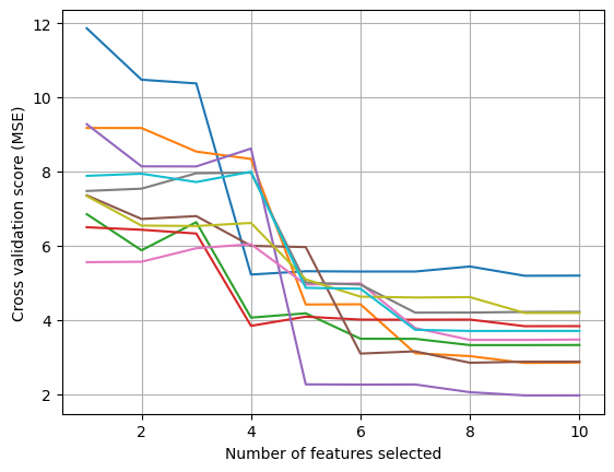
# Plot number of features VS. cross-validation scores
plt.figure()
plt.xlabel("Number of features selected")
plt.ylabel("Cross validation score (MSE)")
scores = np.concatenate(
[
-rfecv.cv_results_["split%s_test_score" % i].reshape(-1, 1)
for i in range(num_folds)
],
axis=1,
)
plt.plot(
range(min_features_to_select, X.shape[1] + min_features_to_select),
scores,
)
plt.grid(True)
plt.show()
Optimal number of features for fold 1: 10
Optimal number of features for fold 2: 9
Optimal number of features for fold 3: 11
Optimal number of features for fold 4: 10
Optimal number of features for fold 5: 11
Optimal number of features for fold 6: 10
Optimal number of features for fold 7: 10
Optimal number of features for fold 8: 11
Optimal number of features for fold 9: 8
Optimal number of features for fold 10: 11
Optimal number of features on average: 10
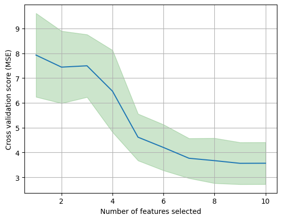
Let us take a look at the mean and standard deviation (variance) of the cross-validation scores for each number of features.
mean_scores = np.mean(scores, axis=1)
std_scores = np.std(scores, axis=1)
plt.figure()
plt.xlabel("Number of features selected")
plt.ylabel("Cross validation score (MSE)")
plt.plot(
    range(min_features_to_select, X.shape[1] + min_features_to_select),
    mean_scores,
)
plt.fill_between(
    range(min_features_to_select, X.shape[1] + min_features_to_select),
    mean_scores - std_scores,
    mean_scores + std_scores,
    alpha=0.2,
    color="g",
)
plt.grid(True)
plt.show()
From the outputs above, we can observe the large variance (inconsistency) across the 10 folds, where the optimal number of features varies from 8 to 11. The variance across folds is also a measure of the stability of the model. The lower the variance, the more stable the model is. Furthermore, if we repeated cross-validation using a different set of cross-validation folds (changing the random seed in np.random.seed(2022) at the top from 2022 to another number), then the precise model with the lowest estimated test error would change.
When there are multiple models with similar cross-validation errors, we can select a model using the one-standard-error rule. We first calculate the standard error of the estimated test MSE for each model size (number of selected features), and then select the smallest model (smallest number of selected features) for which the estimated test error is within one standard error of the lowest point on the curve. The rationale here is that if a set of models appear to be more or less equally good, then we might as well choose the simplest model, i.e. the model with the smallest number of predictors.
6.1.4. Exercises
1. Suppose we have a dataset with \(13\) predictors/features. Now calculate how many models we need to fit for the best subset selection and forward stepwise selection methods.
Compare your answer with the solution below
\(8192\) for best subset selection method and only \(92\) for forward stepwise selection method
2. Forward and backward stepwise selection guarantee the best possible model out of all \(2^D\) models containing subsets of the \(D\) predictors.
   a. True

   b. False
Compare your answer with the solution below
b. False. We can only expect to find a local optimum, not a global optimum.
3. All the following exercises use the Carseats dataset to study feature selection on real-world data.
a. Load the Carseats dataset, convert the values of variables (predictors) from category to numbers, and inspect the first five rows. (Use \(2022\) as the random seed value)
# Write your code below to answer the question
Compare your answer with the reference solution below
import numpy as np
import pandas as pd

np.random.seed(2022)

carseat_url = "https://github.com/pykale/transparentML/raw/main/data/Carseats.csv"

carseat_df = pd.read_csv(carseat_url)
# converting categories
carseat_df["ShelveLoc"] = carseat_df["ShelveLoc"].factorize()[0]
carseat_df["Urban"] = carseat_df["Urban"].factorize()[0]
carseat_df["US"] = carseat_df["US"].factorize()[0]

carseat_df.head(5)
| Sales | CompPrice | Income | Advertising | Population | Price | ShelveLoc | Age | Education | Urban | US | |
|---|---|---|---|---|---|---|---|---|---|---|---|
| 0 | 9.50 | 138 | 73 | 11 | 276 | 120 | 0 | 42 | 17 | 0 | 0 |
| 1 | 11.22 | 111 | 48 | 16 | 260 | 83 | 1 | 65 | 10 | 0 | 0 |
| 2 | 10.06 | 113 | 35 | 10 | 269 | 80 | 2 | 59 | 12 | 0 | 0 |
| 3 | 7.40 | 117 | 100 | 4 | 466 | 97 | 2 | 55 | 14 | 0 | 0 |
| 4 | 4.15 | 141 | 64 | 3 | 340 | 128 | 0 | 38 | 13 | 0 | 1 |
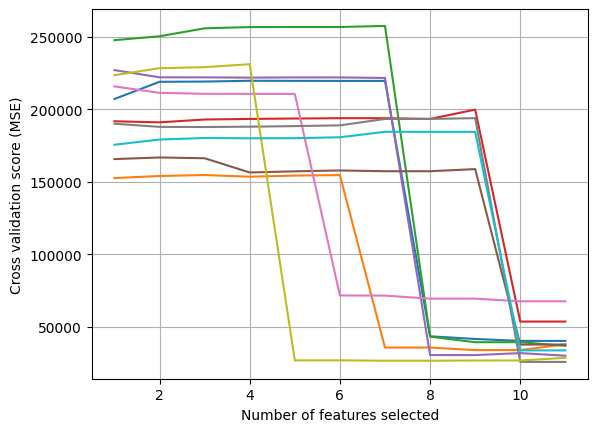
b. Now try to use this pre-processed data from Exercise 3(a) above to perform feature selection for linear regression using scikit-learn’s RFECV API and find the optimal number of features per fold and on average. Finally, plot the number of features selected versus cross-validation scores. Here, the number of folds \(k=10\).
# Write your code below to answer the question
Compare your answer with the reference solution below
import matplotlib.pyplot as plt
from sklearn.feature_selection import RFECV
from sklearn.linear_model import LinearRegression

X = carseat_df.drop(["Sales"], axis=1).values
y = carseat_df.Sales.values

regr = LinearRegression()

min_features_to_select = 1  # Minimum number of features to consider
num_folds = 10
rfecv = RFECV(
    estimator=regr,
    step=1,
    cv=num_folds,
    scoring="neg_mean_squared_error",  # Proportional to the R^2 of the prediction
    min_features_to_select=min_features_to_select,
)
rfecv.fit(X, y)

for i in range(num_folds):
    print(
        "Optimal number of features for fold %d: %d"
        % (i + 1, rfecv.cv_results_["split%d_test_score" % i].argmax() + 1)
    )

print("Optimal number of features on average: %d" % rfecv.n_features_)

# Plot number of features VS. cross-validation scores
plt.figure()
plt.xlabel("Number of features selected")
plt.ylabel("Cross validation score (MSE)")
scores = np.concatenate(
    [
        -rfecv.cv_results_["split%s_test_score" % i].reshape(-1, 1)
        for i in range(num_folds)
    ],
    axis=1,
)
plt.plot(
    range(min_features_to_select, X.shape[1] + min_features_to_select),
    scores,
)
plt.grid(True)
plt.show()
Optimal number of features for fold 1: 9
Optimal number of features for fold 2: 9
Optimal number of features for fold 3: 9
Optimal number of features for fold 4: 9
Optimal number of features for fold 5: 9
Optimal number of features for fold 6: 8
Optimal number of features for fold 7: 8
Optimal number of features for fold 8: 7
Optimal number of features for fold 9: 9
Optimal number of features for fold 10: 8
Optimal number of features on average: 9
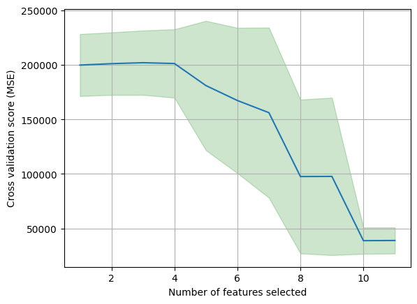
c. Finally, find the mean and standard deviation of the cross-validation scores from Exercise 3(b) above for each number of features.
# Write your code below to answer the question
Compare your answer with the reference solution below
mean_scores = np.mean(scores, axis=1)
std_scores = np.std(scores, axis=1)
plt.figure()
plt.xlabel("Number of features selected")
plt.ylabel("Cross validation score (MSE)")
plt.plot(
    range(min_features_to_select, X.shape[1] + min_features_to_select),
    mean_scores,
)
plt.fill_between(
    range(min_features_to_select, X.shape[1] + min_features_to_select),
    mean_scores - std_scores,
    mean_scores + std_scores,
    alpha=0.2,
    color="g",
)
plt.grid(True)
plt.show()

# From the outputs above, we can observe the some variance (inconsistency) across the 10 folds,
# where the optimal number of features varies from 8 to 10