
Survival Analysis
KaleCancer Example: Clinical covariates and WSI to predict survival
You have a clinical table, a folder of pathology slide features, and follow-up times for each patient.
In this tutorial, we will answer three questions:
Can these data predict who survives longer?
Does combining them beat using either one alone?
What is the model actually looking at, and what does it say about one patient?
The cohort is synthetic. We created the signal ourselves, so we can check that KaleCancer finds it. The results are purely illustrative.
import warnings
import numpy as np
import pandas as pd
import torch
import matplotlib.pyplot as plt
from IPython.display import display

from synthetic_showcase_data import make_showcase_cohort, PATCH_SIZE

RANDOM_STATE = 0

warnings.filterwarnings('ignore', message='IProgress not found')
LOW, HIGH, MODEL = '#2a78d6', '#eb6834', '#1baf7a'
plt.style.use('default')  # Light plots even when the editor uses a dark theme.
plt.rcParams.update({'axes.spines.top': False, 'axes.spines.right': False})
1 Load Your Data
data_folder = '../../../data/synthetic_showcase_survival'
make_showcase_cohort(data_folder, task='survival')

table = pd.read_csv(data_folder + '/clinical.csv', index_col=0)
display(table.head())
| age | gender | time | event | |
|---|---|---|---|---|
| patient_id | ||||
| patient_000 | 63.047171 | M | 140.161953 | True |
| patient_001 | 49.600159 | F | 1862.486595 | True |
| patient_002 | NaN | F | 668.519881 | True |
| patient_003 | 69.405647 | F | 11.549494 | True |
| patient_004 | NaN | F | 2163.788231 | False |
Each patient has a time in days and an event flag. event=True means the event happened at that time. event=False means the patient was censored: they were still event-free when follow-up ended, so all we know is that their event comes later.
Censored patients still carry information, so we don’t drop them. TimeToEvent keeps both columns together, and everything else about loading stays the same.
from kalecancer.loaddata import Tabular, PatchFeatures, TimeToEvent, MultimodalDataset

clinical = Tabular(table.drop(columns=['time', 'event']))
slides = PatchFeatures.from_glob(data_folder + '/patches/*.h5', id_pattern=r'(patient_\d{3})\.h5')
target = TimeToEvent(time=table['time'], event=table['event'])

dataset = MultimodalDataset(
    modalities={'clinical': clinical, 'slides': slides},
    target=target,
    required_modalities=[]
)
display(dataset.summary())
| count | |
|---|---|
| available: clinical | 200 |
| available: slides | 180 |
| available: target | 200 |
| included | 200 |
| included with clinical | 200 |
| included with slides | 180 |
| events | 114 |
Visualising the data
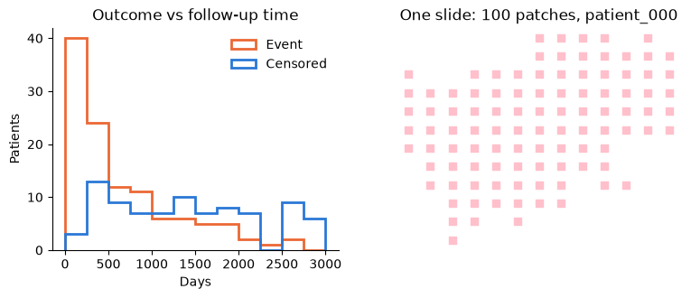
Follow-up ends in one of two ways: an event or censoring. Patches each contain a coordinate pointing to their location on the WSI they encode.
fig, (left, right) = plt.subplots(1, 2, figsize=(9, 3.2))

for event, label, colour in [(True, 'Event', HIGH), (False, 'Censored', LOW)]:
    left.hist(table.loc[table['event'] == event, 'time'], bins=range(0, 3250, 250), histtype='step', linewidth=2, color=colour, label=label)
left.set(title='Outcome vs follow-up time', xlabel='Days', ylabel='Patients')
left.legend(frameon=False)

patient = slides.ids[0]
patches = slides.instances(patient)
right.scatter(patches['x'], patches['y'], marker='s', s=26, color='pink')
right.set_title(f'One slide: {len(patches)} patches, {patient}')
right.axis('off')
plt.show()
2 Build a Model
For Intermediate Fusion: each modality gets an encoder, a fusion method combines them, and a head makes the prediction. Only the head changes from classification.
CoxHead predicts one number per patient, the log_hazard: higher means higher risk. ties='efron' sets how the loss handles patients with the same event time.
from kalecancer.model import ABMIL, MLP, IntermediateFusion, MaskedMean, CoxHead

# Needed to ensure model weights are initialised consistently
torch.manual_seed(RANDOM_STATE)

clinical_encoder = MLP(in_dim=2, hidden_dims=[16], out_dim=16, dropout=0.25)
slide_encoder = ABMIL(in_dim=32, hidden_dim=16, attention_dim=8, dropout=0.25)
head = CoxHead(in_dim=16, ties='efron')

model = IntermediateFusion(
    encoders={'clinical': [clinical_encoder], 'slides': [slide_encoder]},
    fusion=MaskedMean(),
    head=head
)
3 Train
Pipeline works just as it does for classification, with two survival choices:
Batch size: the Cox loss compares each event with the patients still at risk in the same batch, so bigger batches give it more to compare. We use 32 rather than 16.
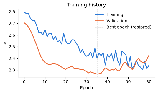
Early stopping: it watches the validation loss rather than a metric like AUROC. The concordance index,
HarrellC, only changes when two patients swap order. With few validation events, it moves in coarse steps and ties between epochs, so we use it to evaluate instead.
from functools import partial
from sklearn.impute import SimpleImputer
from sklearn.model_selection import StratifiedShuffleSplit
from sklearn.preprocessing import OrdinalEncoder, StandardScaler
from kalecancer.pipeline import EarlyStopping, Pipeline
from kalecancer.prepdata import ColumnGroup, TableTransform

clinical_transform = TableTransform(
    groups={
        'numeric': ColumnGroup(['age'], [SimpleImputer(), StandardScaler()]),
        'categorical': ColumnGroup(['gender'], [OrdinalEncoder(encoded_missing_value=-1)])
    },
    drop=[]
)

pipeline = Pipeline(
    model=model,
    transforms={'clinical': clinical_transform},
    optimizer=partial(torch.optim.AdamW, lr=3e-3),
    batch_size=32,
    drop_last=False,
    max_epochs=80,
    validation=StratifiedShuffleSplit(n_splits=1, test_size=0.2, random_state=RANDOM_STATE),
    early_stopping=EarlyStopping(metric='loss', patience=25, restore_best=True),
    accelerator='cpu',
    precision='32-true',
    random_state= RANDOM_STATE
)
Splits are stratified on event, so train and test keep the same share of events.
from kalecancer.loaddata import train_test_split

train, test = train_test_split(dataset, test_size=0.25, stratify=True, random_state=RANDOM_STATE)

pipeline.fit(train)
pipeline.fit_report_
{'n_train': 120,
 'n_val': 30,
 'events': 68,
 'epochs_run': 61,
 'best_epoch': 35,
 'best_score': 2.2644824981689453,
 'optimizer_steps': 244,
 'skipped_batches': 0,
 'non_finite_inputs': {},
 'baseline_events': 85}
fig, ax = plt.subplots(figsize=(6, 3))
ax.plot(pipeline.history_['train_loss'], color=LOW, linewidth=2, label='Training')
ax.plot(pipeline.history_['val_loss'], color=HIGH, linewidth=2, label='Validation')
ax.axvline(pipeline.fit_report_['best_epoch'], color='grey', linestyle='--', linewidth=1, label='Best epoch (restored)')
ax.set(title='Training history', xlabel='Epoch', ylabel='Loss')
ax.legend(frameon=False)
plt.show()
4 Evaluate
A log-hazard only ranks patients, and its zero point is arbitrary. To turn it into survival probabilities, fit also estimates a baseline hazard on the training patients. Pass survival_times to get a survival[<time>] column for each time.
All patients get a prediction, even those that don’t have any patches.
survival_times = [365 * year for year in range(1, 6)]
predictions = pipeline.predict(test, survival_times=survival_times)

no_slide = test.present.index[~test.present['slides']]
print(f'{len(no_slide)} of the {len(test)} test patients have no slide. Their predictions:')
display(predictions.loc[no_slide[:]].round(3))
2 of the 50 test patients have no slide. Their predictions:
| log_hazard | survival[365.0] | survival[730.0] | survival[1095.0] | survival[1460.0] | survival[1825.0] | |
|---|---|---|---|---|---|---|
| id | ||||||
| patient_030 | 1.431 | 0.806 | 0.707 | 0.615 | 0.536 | 0.447 |
| patient_145 | 1.428 | 0.806 | 0.708 | 0.616 | 0.537 | 0.448 |
Survival metrics answer different questions:
Metric |
Question |
Reading it |
|---|---|---|
|
Of two patients, did the one with the earlier event have the higher risk? |
1 is perfect, 0.5 is chance |
|
The same, up to 5 years, weighted to correct for censoring |
1 is perfect, 0.5 is chance |
|
Can it separate who had the event by 3 years from who didn’t? |
1 is perfect, 0.5 is chance |
|
How close are the predicted probabilities to what happened? |
0 is perfect, about 0.25 is predicting 50% for everyone |
|
When we predict 70% survival, do about 70% survive? |
0 is perfect |
|
How far apart are the survival curves of the risk groups? |
Higher is better, about 1 is chance |
The first three only rank patients, so a model can score well on them and still predict the wrong probabilities. IntegratedBrier and CalibrationError check the probabilities too.
from kalecancer.evaluate import CalibrationError, HarrellC, IntegratedBrier, LogRank, TimeDependentAUC, UnoC

harrell = HarrellC()

metrics = {
    'harrell_c': harrell,
    'uno_c_5y': UnoC(tau=365.0*5),
    'auc_3y': TimeDependentAUC(time=365.0*3),
    'integrated_brier': IntegratedBrier(),
    'calibration_error': CalibrationError(n_bins=3),
    'log_rank': LogRank(n_groups=2)
}

pipeline.evaluate(test, metrics, survival_times=survival_times)
harrell_c             0.797657
uno_c_5y              0.782294
auc_3y                0.851631
integrated_brier      0.181243
calibration_error     0.090533
log_rank             14.654722
Name: score, dtype: float64
A C-index can’t reach 1 here, even for a perfect model. Event times are random, so a high-risk patient sometimes outlives a low-risk one. Scoring these test patients with the exact risk formula we used to create them gives about 0.79, which is about what our model scores. With only 50 patients, either one can come out slightly ahead by chance.
Evaluating on the training cohort is data leakage. KaleCancer guards against this behaviour.
try:
    pipeline.evaluate(train, metrics, survival_times=survival_times)
except ValueError as error:
    print(error)
150 patients were used to fit this pipeline (e.g. ['patient_001', 'patient_004', 'patient_005', 'patient_006', 'patient_007']); evaluate on held-out patients, or pass allow_seen=True
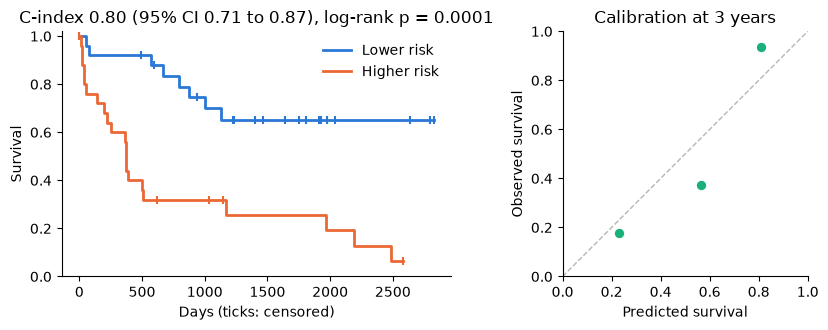
bootstrap_ci allows us to calculate confidence intervals instead of a single metric value.
kaplan_meier splits patients into risk groups by log_hazard and estimates each group’s survival. calibration_table compares predicted survival with observed survival. Observed survival comes from a Kaplan-Meier estimate, so censoring is handled correctly.
from scipy.stats import chi2
from kalecancer.evaluate import EvalContext, bootstrap_ci, calibration_table, kaplan_meier

truth = test.target.frame.loc[predictions.index]
context = EvalContext(train_target=pipeline.train_target_, classes=None)
interval = bootstrap_ci(harrell, predictions, truth, context)

curves = kaplan_meier(predictions, truth, n_groups=2, labels=['Lower risk', 'Higher risk'])
p_value = chi2.sf(metrics['log_rank'](predictions, truth, context), df=1)
calibration = calibration_table(predictions, truth, n_bins=3)
calibration = calibration[calibration['time'] == 1095]

fig, (left, right) = plt.subplots(1, 2, figsize=(9, 3.4))

for group, colour in [('Lower risk', LOW), ('Higher risk', HIGH)]:
    curve = curves[curves['group'] == group]
    censored = curve[(curve['events'] == 0)]
    left.step(curve['time'], curve['survival'], where='post', color=colour, linewidth=2, label=group)
    left.scatter(censored['time'], censored['survival'], marker='|', s=40, color=colour)
left.set(title=f'C-index {interval.estimate:.2f} (95% CI {interval.lower:.2f} to {interval.upper:.2f}), log-rank p = {p_value:.1g}',
         xlabel='Days (ticks: censored)', ylabel='Survival', ylim=(0, 1.02))
left.legend(frameon=False)

right.plot([0, 1], [0, 1], color='#b8b6ae', linestyle='--', linewidth=1)
right.scatter(calibration['expected'], calibration['observed'], s=60, color=MODEL, edgecolor='white')
right.set(title='Calibration at 3 years', xlabel='Predicted survival', ylabel='Observed survival', xlim=(0, 1), ylim=(0, 1))
right.set_aspect('equal')
plt.tight_layout()
plt.show()
5 Does Combining Modalities Help?
Swapping the model takes one line, and everything else stays the same. To compare fairly, we use only patients who have both modalities, and train every candidate for the same number of epochs.
For survival, late fusion needs this anyway. Each branch’s log-hazard has an arbitrary offset, so averaging different branches for different patients would reorder them. KaleCancer refuses to fit it on patients with a missing slide:
from sklearn.base import clone
from kalecancer.model import LateFusion, Unimodal

clinical_model = Unimodal('clinical', [clinical_encoder], head)
slide_model = Unimodal('slides', [slide_encoder], head)
late_fusion = LateFusion({'clinical': clinical_model, 'slides': slide_model}, fusion=MaskedMean())

try:
    clone(pipeline).set_params(model=late_fusion).fit(train)
except ValueError as error:
    print(error)
MaskedMean over Cox Head needs every patient to have every branch, but 18 do not: each branch's log-hazard has an arbitrary offset, so averaging different subsets of branches would reorder patients
cross_validate refits everything in every fold:
from sklearn.model_selection import StratifiedKFold
from kalecancer.evaluate import cross_validate

candidates = {
    'Clinical only': clinical_model,
    'Slides only': slide_model,
    'Late fusion': late_fusion,
    'Intermediate fusion': model
}

complete = dataset.subset(dataset.present_ids('slides'))
folds = StratifiedKFold(n_splits=3, shuffle=True, random_state=RANDOM_STATE)
fixed_training = {'validation': None, 'early_stopping': None, 'max_epochs': 40}

results = {
    name: cross_validate(clone(pipeline).set_params(model=candidate, **fixed_training), complete, folds, {'harrell_c': harrell})
    for name, candidate in candidates.items()
}
fig, ax = plt.subplots(figsize=(7, 2.8))
for row, (name, result) in enumerate(results.items()):
    scores = result.folds['harrell_c']
    ax.scatter(scores, [row] * len(scores), s=45, color=MODEL, alpha=0.6, edgecolor='none', label='One fold' if row == 0 else None)
    ax.scatter(scores.mean(), row, s=160, marker='|', color='#2b2a27', linewidth=2, label='Mean' if row == 0 else None)
    ax.annotate(f'{scores.mean():.2f}', (scores.mean(), row), xytext=(0, 9), textcoords='offset points', ha='center')
ax.set_yticks(range(len(results)), results.keys())
ax.set_ylim(-0.6, len(results) - 0.3)
ax.set(title='Cross-validated C-index', xlabel='C-index', xlim=(0.4, 1))
ax.legend(frameon=False, loc='upper left')
plt.show()
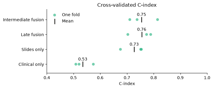
From the above we can see that slides do most of the predictive work.
Given a baseline, bootstrap_ci scores both models on the same resampled patients, so the interval is of the gain itself.
clinical_pipeline = clone(pipeline).set_params(model=clinical_model, **fixed_training).fit(train)
clinical_predictions = clinical_pipeline.predict(test)

gain = bootstrap_ci(
    harrell, predictions, truth, context,
    baseline=clinical_predictions
)
print(f'C-index gained by adding slides to the clinical table: {gain.estimate:+.2f} (95% CI {gain.lower:+.2f} to {gain.upper:+.2f})')
C-index gained by adding slides to the clinical table: +0.27 (95% CI +0.13 to +0.41)
6 Interpreting the results
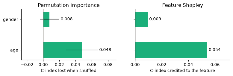
The cohort was synthesised with these signals: slides carry the most signal, age adds some, and gender adds none.
Can the interpretation tools recover them?
6.1 Which modality matters?
These tools mark a modality as absent and measure what the model loses. Each modality is scored on the same patients, so the patients with no slide are left out.
from kalecancer.interpret import leave_one_out_ablation, modality_shapley

shapley = modality_shapley(pipeline, test, harrell)
ablation = leave_one_out_ablation(pipeline, test, harrell)

print(f"Scored on {len(test) - shapley.attrs['n_excluded']} patients")
pd.DataFrame({'Shapley value': shapley, 'C-index lost when removed': ablation}).round(3)
Scored on 48 patients
| Shapley value | C-index lost when removed | |
|---|---|---|
| clinical | 0.031 | 0.031 |
| slides | 0.245 | 0.245 |
Note: with two modalities, Shapley and ablation match. With three or more, Shapley also splits the credit fairly between modalities that overlap.
6.2 Which clinical features matter?
from kalecancer.interpret import feature_shapley, permutation_importance

importance = permutation_importance(pipeline, test, harrell, n_repeats=20, seed=RANDOM_STATE)
feature_values = feature_shapley(pipeline, test, harrell, n_samples=30, seed=RANDOM_STATE)

fig, (left, right) = plt.subplots(1, 2, figsize=(9, 2.2), sharey=True)
left.barh(importance.index, importance['mean'], xerr=importance['std'], color=MODEL, height=0.5)
left.set(title='Permutation importance', xlabel='C-index lost when shuffled')
right.barh(feature_values.index, feature_values, color=MODEL, height=0.5)
right.set(title='Feature Shapley', xlabel='C-index credited to the feature')
for ax in (left, right):
    ax.bar_label(ax.containers[-1], fmt='%.3f', padding=4)
    ax.axvline(0, color='#8a8880', linewidth=1)
    ax.margins(x=0.32)
plt.show()
6.3 Where on the slide?
attention shows us how much weight the model gave every patch, and attention_heatmap helps us visualise these values.
Our synthetic data records which patches are truly aggressive, so we can compare the two.
import h5py
from kalecancer.interpret import attention, attention_heatmap, save_heatmap

weights = attention(pipeline, test, 'slides')

def read_aggressive(path):
    with h5py.File(path) as f:
        return f['aggressive'][:]

weights['aggressive'] = np.concatenate([read_aggressive(path) for path in weights['file'].unique()])
weights.drop(columns='file').head()
| patient_id | x | y | attention | aggressive | |
|---|---|---|---|---|---|
| 0 | patient_000 | 0 | 1280 | 0.003052 | False |
| 1 | patient_000 | 0 | 1536 | 0.005476 | False |
| 2 | patient_000 | 0 | 1792 | 0.013401 | False |
| 3 | patient_000 | 0 | 2048 | 0.006105 | False |
| 4 | patient_000 | 0 | 2304 | 0.004948 | False |
def heatmap(patient, column):
    rows = weights[weights['patient_id'] == patient]
    return attention_heatmap(rows, patch_size=PATCH_SIZE, downsample=2 * PATCH_SIZE, weight_column=column)

patients = predictions.loc[test.present_ids('slides'), 'log_hazard'].nlargest(3).index

fig, axes = plt.subplots(2, 3, figsize=(9, 6))
for column, patient in enumerate(patients):
    axes[0, column].imshow(heatmap(patient, 'aggressive'), cmap='Oranges', vmin=-0.15)
    axes[0, column].set_title(patient)
    axes[1, column].imshow(heatmap(patient, 'attention'), cmap='Oranges', vmin=-0.15)
for ax in axes.flat:
    ax.set(xticks=[], yticks=[])
    ax.spines[:].set_visible(False)
axes[0, 0].set_ylabel('Truly aggressive')
axes[1, 0].set_ylabel('Model attention')
plt.tight_layout()
plt.show()
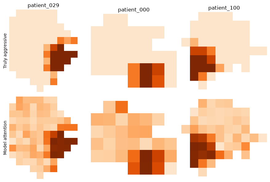
Those three are the model’s highest-risk patients, so here is the check across every test slide: for each one, are the patches it attends to most actually aggressive?
def hit_rate(rows):
    return rows.nlargest(rows['aggressive'].sum(), 'attention')['aggressive'].mean()

with_region = weights.groupby('patient_id').filter(lambda rows: rows['aggressive'].any())
hits = with_region.groupby('patient_id')[['attention', 'aggressive']].apply(hit_rate)
chance = with_region.groupby('patient_id')['aggressive'].mean()

print(f'Most-attended patches that are truly aggressive: {hits.mean():.0%} (chance: {chance.mean():.0%}, {len(hits)} slides)')
Most-attended patches that are truly aggressive: 100% (chance: 10%, 47 slides)
Save the results to review them outside Python: a PNG for each heatmap, and a table of weights and coordinates.
save_heatmap(heatmap(patients[0], 'attention'), data_folder + f'/heatmaps/{patients[0]}.png', colormap='Oranges')
weights.to_csv(data_folder + '/heatmaps/attention.csv', index=False)
6.4 What has it learned?
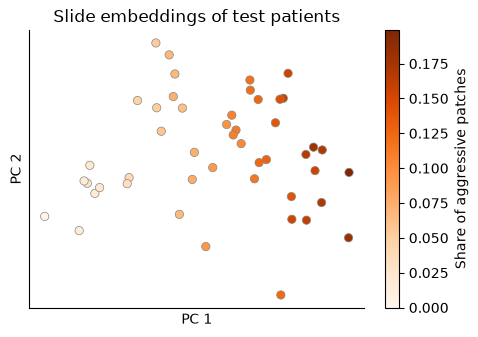
encode gives you the embedding of any modality, ready for your own analysis. Survival has no classes to colour by, so we colour each patient by the true share of aggressive patches on their slide.
from sklearn.decomposition import PCA

embeddings = pipeline.encode(test, 'slides')
projection = PCA(n_components=2).fit_transform(embeddings)
aggressive_share = weights.groupby('patient_id')['aggressive'].mean().loc[embeddings.index]

fig, ax = plt.subplots(figsize=(5.4, 3.6))
points = ax.scatter(*projection.T, c=aggressive_share, cmap='Oranges', vmin=0, s=36, edgecolor='#8a8880', linewidth=0.5)
ax.set(title='Slide embeddings of test patients', xlabel='PC 1', ylabel='PC 2', xticks=[], yticks=[])
fig.colorbar(points, label='Share of aggressive patches')
plt.show()
6.5 What about one patient?
Everything above describes the cohort. patient_report explains one patient’s own prediction: their risk, their survival curve, what pushed their risk up or down, and which patches mattered.
Here are the highest and lowest risk test patients who have a slide.
from kalecancer.interpret import patient_report, save_reports

risk = predictions.loc[test.present_ids('slides'), 'log_hazard']
highest, lowest = risk.idxmax(), risk.idxmin()

reports = patient_report(pipeline, dataset, [highest, lowest], survival_times=list(range(0, 1826, 25)), seed=RANDOM_STATE)

display(table.loc[[highest, lowest], ['age', 'gender']].round(1))
display(pd.DataFrame({
    report.patient_id: {
        'log-hazard': report.risk,
        'risk percentile': report.risk_percentile,
        **report.modality_contributions.add_prefix('modality: ').to_dict(),
        **report.feature_contributions.add_prefix('feature: ').to_dict()
    }
    for report in reports
}).round(2))
| age | gender | |
|---|---|---|
| patient_id | ||
| patient_029 | 64.3 | M |
| patient_058 | 51.3 | F |
| patient_029 | patient_058 | |
|---|---|---|
| log-hazard | 3.18 | -0.01 |
| risk percentile | 98.75 | 7.25 |
| modality: clinical | -1.02 | 1.23 |
| modality: slides | 1.02 | -1.23 |
| feature: age | 0.24 | -0.14 |
| feature: gender | 0.14 | 0.05 |
fig, ax = plt.subplots(figsize=(6, 3))
for report, label, colour in zip(reports, ['Highest risk', 'Lowest risk'], [HIGH, LOW], strict=True):
    ax.plot(report.survival['time'], report.survival['survival'], color=colour, linewidth=2, label=f'{label}: {report.patient_id}')
ax.set(title='Predicted survival of two patients', xlabel='Days', ylabel='Survival', ylim=(0, 1.02))
ax.legend(frameon=False)
plt.show()
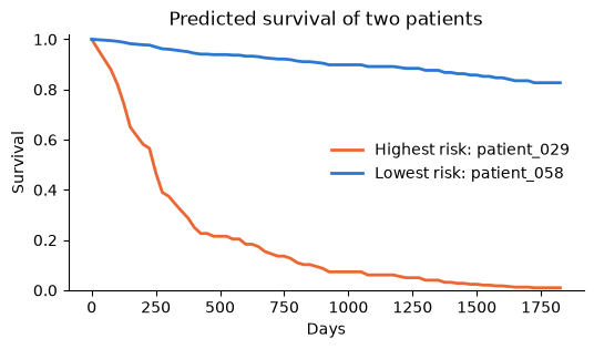
These are changes in this patient’s own log-hazard, not the cohort-level scores from 6.1 and 6.2.
Each report also lists the patient’s most-attended patches, so you can find them on the slide:
display(reports[0].top_patches.drop(columns='file').head(3))
save_reports(reports, data_folder + '/patient_reports.json')
| x | y | attention | |
|---|---|---|---|
| 0 | 3072 | 2816 | 0.009703 |
| 1 | 3072 | 3584 | 0.009668 |
| 2 | 3072 | 3072 | 0.009658 |
KaleCancer Workflow
You want to |
Use |
|---|---|
Join a table and slides by patient |
|
Prepare data |
|
Try different models |
|
Measure ranking |
|
Measure predicted probabilities |
|
Compare risk groups |
|
Get confident estimates |
|
Explain modalities and features |
|
Interpret slides |
|
Explain one patient |
|
Share the experiment |
|
There is more beyond this notebook:
Classification outcomes:
ClassificationHead,AUROCandBalancedAccuracy, inclassification_showcase.ipynb.Real slides:
overlay_on_slidedraws a heatmap on the slide image.Larger clinical tables:
TabICLEncoderis a pretrained tabular encoder.