Cardiothoracic Abnormality Assessment

In this tutorial, we will use PyKale [1] to pretrain, fine-tune, evaluate, and interpret deep learning models on two low-cost, non-invasive data modalities: Chest X-ray (CXR) and 12-lead Electrocardiogram (ECG), for classifying individuals as healthy or having a cardiothoracic abnormality.

We will work with a multimodal dataset derived from MIMIC-CXR [2,3] and MIMIC-IV-ECG [4], which contains approximately 50,000 paired CXR–ECG samples.

This tutorial is based on the work of Suvon et al. (MICCAI 2024) [5], which proposed a tri-stream pretraining method using a Multimodal Variational Autoencoder (VAE) to learn both modality-specific and modality-shared representations for estimating Pulmonary Arterial Wedge Pressure (PAWP)—a key indicator of cardiac hemodynamics.

The multimodal approach used in this tutorial involves intermediate fusion, where imaging (CXR) and ECG features are combined at feature embedding level.

The main tasks of this tutorial are:

• Load CXR and ECG data.

• Pretrain a multimodal CardioVAE model using ~49,000 CXR–ECG pairs via a tri-stream pretraining method

• Fine-tune the pretrained CardioVAE model on a smaller subset (~1,000 paired samples) with binary labels: Healthy and Cardiothoracic Abnormality

• Evaluate the performance of the fine-tuned model

• Interpret the trained CardioVAE model across both CXR and ECG modalities

Estimated runtime: Completing the tasks in this tutorial will take approximately 10 minutes (GPU is required).

Step 0: Environment Preparation

Setup Google Colab runtime type

To run this tutorial in Google Colab, you need to use GPU runtime type. Click on the “Runtime” option in the top-left menu, then select “Change runtime type” and choose T4 GPU as the hardware accelerator.

Package installation

The main packages required (excluding PyKale) for this tutorial are:

• wfdb: A toolkit for reading, writing, and processing physiological signal data, especially useful for ECG waveform analysis.

• yacs: A lightweight configuration management library that helps organize experimental settings in a structured, readable format.

• pytorch-lightning: A high-level framework built on PyTorch that simplifies training workflows, making code cleaner and easier to scale.

• tabulate: Used to print tabular data in a readable format, helpful for summarizing results or configuration parameters.

Estimated runtime: 4 minutes

Show code cell source

Hide code cell source

%%capture
!pip install --quiet \
    "pykale[example]@git+https://github.com/pykale/pykale@main" \
    torch-geometric==2.6.0 torch_sparse torch_scatter \
    -f https://data.pyg.org/whl/torch-2.6.0+cu124.html

Setup

As a starting point, we will mount Google Drive in Colab so that the data can be accessed directly. You might be prompted to grant permission to access your Google account—please proceed with the authorisation when asked.

Show code cell source

Hide code cell source

# Connect with your google drive for data and model loading
from google.colab import drive

drive.mount("/content/drive")

Show code cell output

Hide code cell output

Mounted at /content/drive

Next, we will install the required packages and load a set of helper functions to support the tutorial workflow. To keep the output clean and focused on interpretation, we also suppress unnecessary warnings.

Estimated runtime: 25 seconds

Show code cell source

Hide code cell source

import os
import site
import sys
import warnings
import logging


# Disable warnings
warnings.filterwarnings("ignore")
os.environ["PYTHONWARNINGS"] = "ignore"

# Suppress PyTorch Lightning logs
logging.getLogger("pytorch_lightning").setLevel(logging.ERROR)
logging.getLogger("pytorch_lightning.utilities.rank_zero").setLevel(logging.ERROR)
logging.getLogger("pytorch_lightning.accelerators.cuda").setLevel(logging.ERROR)

if "google.colab" in str(get_ipython()):
    sys.path.insert(0, site.getusersitepackages())
    !git clone -q --single-branch -b main https://github.com/pykale/mmai-tutorials
    %cp -r /content/mmai-tutorials/tutorials/cardiac-abnormality-assessment/* /content/
    %rm -r /content/mmai-tutorials

Configuration

To maintain a clean and modular notebook design, CardioVAE uses dedicated configuration files for both pre-training and fine-tuning. This setup ensures a clear separation between code and experimental settings, enhancing reproducibility and flexibility across different tasks and datasets.

Configuration parameters can be overridden using external YAML files (e.g., experiments/pretraining_base.yml, experiments/finetune_base.yml).

Pre-training Configuration

Default settings for the pre-training stage are defined in config_pretrain.py. These include data paths, model architecture, and optimizer parameters. This modular structure allows easy experiment tracking and customisation by simply editing the associated .yml file.

from config_pretrain import get_cfg_defaults

cfg_PT = get_cfg_defaults()
cfg_PT.merge_from_file("configs/pretraining_base.yml")

# ------ Hyperparameters to play with -----
cfg_PT.MODEL.LATENT_DIM = 128
cfg_PT.TRAIN.EPOCHS = 1
cfg_PT.TRAIN.LAMBDA_IMAGE = 1
cfg_PT.TRAIN.LAMBDA_SIGNAL = 10
# User can change this to try different batch size.
cfg_PT.DATA.BATCH_SIZE = 128

print(cfg_PT)

DATA:
  BATCH_SIZE: 128
  CXR_PATH: /content/drive/MyDrive/EMBC_workshop_data/cxr_features_tensor_1000.pt
  ECG_PATH: /content/drive/MyDrive/EMBC_workshop_data/ecg_features_tensor_1000.pt
  NUM_WORKERS: 2
MODEL:
  INPUT_DIM_CXR: 1
  INPUT_DIM_ECG: 60000
  LATENT_DIM: 128
  NUM_LEADS: 12
TRAIN:
  ACCELERATOR: gpu
  DATA_DEVICE: cpu
  DEVICE: cuda
  DEVICES: 1
  EPOCHS: 1
  LAMBDA_IMAGE: 1
  LAMBDA_SIGNAL: 10
  LR: 0.001
  SAVE_PATH: cardioVAE.pth
  SCALE_FACTOR: 0.0001
  SEED: 123

Fine-tuning Configuration

Fine-tuning parameters are managed in config_finetune.py. These include learning rate, loss weights, number of epochs, model checkpoint paths, and other task-specific options. External YAML files like experiments/finetune_base.yml enable flexible adjustments for different downstream tasks or datasets.

from config_finetune import get_cfg_defaults

cfg_FT = get_cfg_defaults()
cfg_FT.merge_from_file("configs/finetune_base.yml")

# ------ Hyperparameters to play with -----
cfg_FT.FT.EPOCHS = 10
cfg_FT.FT.HIDDEN_DIM = 128
# User can change this to try different batch size.
cfg_FT.DATA.BATCH_SIZE = 32

print(cfg_FT)

DATA:
  BATCH_SIZE: 32
  CSV_PATH: /content/drive/MyDrive/EMBC_workshop_data/chexpert_healthy_abnormality_subset.csv
  CXR_PATH: /content/drive/MyDrive/EMBC_workshop_data/cxr_features_tensor_last_1000.pt
  DATA_DEVICE: cpu
  ECG_PATH: /content/drive/MyDrive/EMBC_workshop_data/ecg_features_tensor_last_1000.pt
  NUM_WORKERS: 2
FT:
  ACCELERATOR: gpu
  CKPT_PATH: /content/drive/MyDrive/EMBC_workshop_data/CardioVAE.pth
  DEVICE: cuda
  DEVICES: 1
  EPOCHS: 10
  HIDDEN_DIM: 128
  KFOLDS: 5
  LR: 0.001
  NUM_CLASSES: 2
  SEED: 42
INTERPRET:
  CXR_THRESHOLD: 0.7
  ECG_THRESHOLD: 0.7
  SAMPLE_IDX: 101
  SAMPLING_RATE: 500
  ZOOM_RANGE: [3, 3.5]
MODEL:
  INPUT_DIM_ECG: 60000
  INPUT_IMAGE_CHANNELS: 1
  LATENT_DIM: 256
  NUM_LEADS: 12

Step 1: Data Loading and Preparation

This tutorial uses separate data pipelines for pre-training and fine-tuning, both based on paired chest X-ray (CXR) and ECG signal features. Each stage follows standard preprocessing steps—such as resizing, normalization, interpolation, and tensor conversion—tailored for resource-constrained environments like Google Colab.

PyKale API for Data preparation:

• kale.loaddata.signal_access.load_ecg_from_folder provides a convenient function for loading ECG waveform data stored in a directory structure. It supports automatic parsing and conversion of ECG signal files into PyTorch tensors, with options for standard preprocessing such as normalisation, resize, interpolation, and resampling. This enables streamlined integration with deep learning pipelines.

• kale.loaddata.image_access.load_images_from_dir offers an easy-to-use utility for loading image datasets from directory hierarchies. It supports standard image formats and returns PyTorch tensors, performing essential preprocessing steps such as resizing and normalisation. This function is suitable for image classification, computer vision, and multimodal learning tasks.

• kale.loaddata.signal_image_access.SignalImageDataset defines a unified dataset class designed for paired signal (e.g., ECG) and image (e.g., CXR) modalities. It facilitates synchronized access to multi-source data, providing ready-to-use PyTorch datasets that can be directly utilised for multimodal training, evaluation, and downstream applications.

Note: Please create a shortcut to the following Google Drive folder in your MyDrive. To create a shortcut: (i) Click the link to open the Google Drive folder. (ii) Click the folder name at the top to reveal a drop-down menu. (iii) From the drop-down menu, select Organise > Add shortcut. (iv) A dialog box titled “Add shortcut to ‘EMBC_workshop_data’” will appear — click the “All locations” tab, then select “My Drive”. (v) A shortcut to EMBC_workshop_data should now be visible at https://drive.google.com/drive/my-drive.

Google Drive Link

There’s no need to download the data manually. After mounting your Google Drive in the setup section, you will be able to directly access all datasets and pretrained models.

Pre-training Data Loading

To accommodate the resource constraints of platforms like Google Colab, this tutorial uses a lightweight version of the dataset consisting of the first 1,000 preprocessed samples from the full 50K paired CXR and ECG dataset. This significantly reduces runtime and memory requirements, allowing for rapid experimentation without the overhead of full-scale data loading and transformation.

The complete preprocessing pipeline, implemented using the PyKale API, is provided for reference. Additionally, CSV files containing subject IDs for the full dataset are provided. Users interested in training on the complete 50K dataset can leverage the PyKale API, which supports direct loading of raw CXR and ECG features with integrated preprocessing.

Note:

• For ease of use in Colab, the full data loading functionality is commented out by default. It can be re-enabled for local or high-resource environments. To load the full 50K paired CXR-ECG data, you need to download the MIMIC-CXR and MIMIC-IV-ECG datasets, then uncomment the optional code cell and run it.

• To access the required files for dataloading, ensure that the shared folder EMBC_workshop_data is added as a shortcut to your Google Drive (under “My Drive”).

Estimated runtime: 12 seconds

# (OPTIONAL)
# from kale.loaddata.signal_access import load_ecg_from_folder
# from kale.loaddata.image_access import load_images_from_dir

# ecg_tensor = load_ecg_from_folder("/mimic-iv-ecg-diagnostic-electrocardiogram-matched-subset-1.0/", "mimic_ecg_50K.csv")
# cxr_tensor = load_images_from_dir("/physionet.org/files/mimic-cxr-jpg/2.0.0/", "mimic_cxr_50K.csv")

# train_dataset_PT, val_dataset_PT = SignalImageDataset.prepare_data_loaders( ecg_tensor, cxr_tensor)

import torch
from kale.loaddata.signal_image_access import SignalImageDataset
from kale.utils.seed import set_seed
import random
import numpy as np
import torch

set_seed(cfg_PT.TRAIN.SEED)

ecg_tensor_PT = torch.load(cfg_PT.DATA.ECG_PATH, map_location=cfg_PT.TRAIN.DATA_DEVICE)
cxr_tensor_PT = torch.load(cfg_PT.DATA.CXR_PATH, map_location=cfg_PT.TRAIN.DATA_DEVICE)

train_dataset_PT, val_dataset_PT = SignalImageDataset.prepare_data_loaders(
    ecg_tensor_PT, cxr_tensor_PT
)

Fine-tuning Data Loading

For the fine-tuning stage, we use the last 1,000 paired CXR and ECG samples from the full 50K dataset derived from MIMIC-CXR and MIMIC-IV-ECG. Corresponding disease labels are obtained from MIMIC-CXR, which includes 12 cardiothoracic abnormality classes along with a “No Finding” label representing healthy cases.

To formulate a binary classification task, all abnormality classes are grouped into a single Cardiothoracic Abnormality category, while the “No Finding” label is treated as Healthy. The resulting label mapping is as follows:

• 0: Healthy

• 1: Cardiothoracic Abnormality

This fine-tuning subset is explicitly selected to ensure no overlap with the samples used during pre-training, thereby simulating a realistic downstream evaluation setting.

Unlike the fine-tuning strategy reported in Suvon et al., MICCAI 2024, which relied on a private in-house dataset, this approach is fully reproducible using publicly available data from MIMIC-CXR and MIMIC-IV-ECG.

Estimated runtime: 10 seconds

import torch
from torch.utils.data import TensorDataset, DataLoader, random_split
import pandas as pd

# Set seed for reproducibility
torch.manual_seed(cfg_FT.FT.SEED)

# Load data
ecg_tensor_FT = torch.load(cfg_FT.DATA.ECG_PATH, map_location=cfg_FT.DATA.DATA_DEVICE)
cxr_tensor_FT = torch.load(cfg_FT.DATA.CXR_PATH, map_location=cfg_FT.DATA.DATA_DEVICE)
label_df = pd.read_csv(cfg_FT.DATA.CSV_PATH)
labels = torch.tensor(label_df["label"].values, dtype=torch.long)

# Combine tensors into a single dataset
dataset = TensorDataset(cxr_tensor_FT, ecg_tensor_FT, labels)

# Split into train/val
val_ratio = 0.2
num_samples = len(dataset)
num_val = int(val_ratio * num_samples)
num_train = num_samples - num_val

train_dataset_FT, val_dataset_FT = random_split(
    dataset,
    [num_train, num_val],
    generator=torch.Generator().manual_seed(cfg_FT.FT.SEED),
)

# DataLoaders
train_loader_FT = DataLoader(
    train_dataset_FT,
    batch_size=cfg_FT.DATA.BATCH_SIZE,
    shuffle=True,
    num_workers=cfg_FT.DATA.NUM_WORKERS,
)
val_loader_FT = DataLoader(
    val_dataset_FT,
    batch_size=cfg_FT.DATA.BATCH_SIZE,
    shuffle=False,
    num_workers=cfg_FT.DATA.NUM_WORKERS,
)

Step 2: Model Definition

We use the PyKale library to implement a modular multimodal variational autoencoder (VAE) for learning joint representations from ECG and CXR data. The architecture includes modality-specific encoders and decoders, a PoE-based fusion mechanism, and task-specific heads for reconstruction and classification.

Embed

The embedding module is composed of independent encoders for each modality and a fusion mechanism to obtain a shared latent representation.

Signal Encoder

The ECG signal pathway uses SignalVAEEncoder from kale.embed.signal_cnn. This encoder captures high-level temporal features from preprocessed ECG waveforms and maps them to a latent space suitable for downstream fusion and representation learning.

Image Encoder

The image pathway uses ImageVAEEncoder from kale.embed.image_cnn. This encoder captures high-level spatial features from preprocessed CXR’s and maps them to a latent space suitable for downstream fusion and representation learning.

Feature Fusion

Encoded modality-specific features are combined using a Product-of-Experts (PoE) approach, implemented in kale.embed.feature_fusion. The PoE fusion computes a joint posterior over the latent space by aggregating information from each modality, enabling coherent multimodal representation.

Predict

Reconstruction (Pre-training)

During pre-training, the model reconstructs both modalities using decoders from the shared latent representation:

• ImageVAEDecoder from kale.predict.decode for CXR reconstruction

• SignalVAEDecoder from kale.predict.decode for ECG waveform reconstruction

The model is trained to minimise the Evidence Lower Bound (ELBO), encouraging informative and disentangled latent representations.

Classification (Fine-tuning)

For downstream classification tasks, we reuse the pretrained encoders as feature extractors. The SignalImageFineTuningClassifier from kale.predict.decode adds a lightweight classification head on top of the shared latent space for supervised learning. This setup is optimised for clinical prediction tasks, such as binary or multi-label disease classification.

Step 3: Model Training

Multimodal Pretraining

We pretraind a CardioVAE model using the SignalImageVAE class from PyKale to jointly model paired CXR and ECG data. The goal is to learn shared and modality-specific representations in an unsupervised manner via reconstruction.

We instantiate SignalImageVAE from kale.embed.multimodal_encoder, which includes:

• A signal encoder-decoder built on SignalVAEEncoder for ECG waveforms

• An image encoder-decoder built on ImageVAEEncoder for CXR images

• A Product-of-Experts (PoE) fusion module for combining modality-specific latent vectors into a shared latent representation

To pretrain, we use SignalImageTriStreamVAETrainer from kale.pipeline.multimodal_trainer to:

• Perform joint and single-modality reconstructions

• Optimise the ELBO loss, balancing image and signal modalities

• Manage logging, and reconstruction-based validation

Estimated runtime: 2 minutes with 1 epoch

import pytorch_lightning as pl
from kale.pipeline.multimodal_trainer import SignalImageTriStreamVAETrainer
from kale.embed.multimodal_encoder import SignalImageVAE

model = SignalImageVAE(
    image_input_channels=cfg_PT.MODEL.INPUT_DIM_CXR,
    signal_input_dim=cfg_PT.MODEL.INPUT_DIM_ECG,
    latent_dim=cfg_PT.MODEL.LATENT_DIM,
)

# PyKale trainer instance (all from config)
pl_trainer = SignalImageTriStreamVAETrainer(
    model=model,
    train_dataset=train_dataset_PT,
    val_dataset=val_dataset_PT,
    batch_size=cfg_PT.DATA.BATCH_SIZE,
    num_workers=cfg_PT.DATA.NUM_WORKERS,
    lambda_image=cfg_PT.TRAIN.LAMBDA_IMAGE,
    lambda_signal=cfg_PT.TRAIN.LAMBDA_SIGNAL,
    lr=cfg_PT.TRAIN.LR,
    annealing_epochs=cfg_PT.TRAIN.EPOCHS,
    scale_factor=cfg_PT.TRAIN.SCALE_FACTOR,
)

trainer = pl.Trainer(
    max_epochs=cfg_PT.TRAIN.EPOCHS,
    accelerator=cfg_PT.TRAIN.ACCELERATOR,
    devices=cfg_PT.TRAIN.DEVICES,
    log_every_n_steps=10,
)

trainer.fit(pl_trainer)

# Save model state dict
torch.save(model.state_dict(), cfg_PT.TRAIN.SAVE_PATH)
print(f"Saved model state dictionary to '{cfg_PT.TRAIN.SAVE_PATH}'")

INFO:pytorch_lightning.callbacks.model_summary:
  | Name  | Type           | Params | Mode 
-------------------------------------------------
0 | model | SignalImageVAE | 204 M  | train
-------------------------------------------------
204 M     Trainable params
0         Non-trainable params
204 M     Total params
816.722   Total estimated model params size (MB)
32        Modules in train mode
0         Modules in eval mode

Saved model state dictionary to 'cardioVAE.pth'

Multimodal Fine-tuning

For downstream classification, we fine-tune a shallow classifier on top of a pretrained CardioVAE encoder. The encoder is loaded from SignalImageVAE, pretrained with reconstruction loss, and used as a fixed or partially trainable feature extractor.

We use SignalImageFineTuningTrainer from kale.pipeline.multimodal_trainer, which wraps:

• A pretrained CardioVAE model

• A SignalImageFineTuningClassifier (two-layer fully connected classifier)

• A training step that supports standard supervised learning with cross-entropy loss

Estimated runtime: 2 minute with 10 epoch

import torch
import pytorch_lightning as pl
from kale.embed.multimodal_encoder import SignalImageVAE
from kale.pipeline.multimodal_trainer import SignalImageFineTuningTrainer
from kale.utils.remap_model_parameters import remap_state_dict_keys

# Load and remap checkpoint
checkpoint = torch.load(cfg_FT.FT.CKPT_PATH, map_location=cfg_FT.FT.DEVICE)
checkpoint = remap_state_dict_keys(checkpoint)

pretrained_mvae = SignalImageVAE(
    image_input_channels=cfg_FT.MODEL.INPUT_IMAGE_CHANNELS,
    signal_input_dim=cfg_FT.MODEL.INPUT_DIM_ECG,
    latent_dim=cfg_FT.MODEL.LATENT_DIM,
)
pretrained_mvae.load_state_dict(checkpoint, strict=False)
pretrained_mvae.to(cfg_FT.FT.DEVICE)
pretrained_mvae.eval()

model_pl = SignalImageFineTuningTrainer(
    pretrained_model=pretrained_mvae,
    num_classes=cfg_FT.FT.NUM_CLASSES,
    lr=cfg_FT.FT.LR,
    hidden_dim=cfg_FT.FT.HIDDEN_DIM,
)

trainer = pl.Trainer(
    max_epochs=cfg_FT.FT.EPOCHS,
    accelerator=cfg_FT.FT.ACCELERATOR,
    devices=cfg_FT.FT.DEVICES,
    log_every_n_steps=10,
    enable_checkpointing=False,
    logger=False,
)

trainer.fit(model_pl, train_dataloaders=train_loader_FT, val_dataloaders=val_loader_FT)

INFO:pytorch_lightning.callbacks.model_summary:
  | Name         | Type                            | Params | Mode 
-------------------------------------------------------------------------
0 | model        | SignalImageFineTuningClassifier | 271 M  | train
1 | val_accuracy | BinaryAccuracy                  | 0      | train
2 | val_auc      | BinaryAUROC                     | 0      | train
3 | val_mcc      | BinaryMatthewsCorrCoef          | 0      | train
-------------------------------------------------------------------------
65.9 K    Trainable params
271 M     Non-trainable params
271 M     Total params
1,086.193 Total estimated model params size (MB)
9         Modules in train mode
16        Modules in eval mode

Step 4: Evaluation

After training, we extract key validation metrics using PyTorch Lightning’s built-in callback_metrics. These metrics provide a quantitative summary of model performance on the validation set.

We report the following:

• Accuracy: Proportion of correct predictions

• AUROC: Area under the Receiver Operating Characteristic curve, measuring ranking quality

• MCC: Matthews Correlation Coefficient, a balanced metric even for imbalanced classes

The metrics are printed in a tabulated format using the tabulate library for clear presentation.

from tabulate import tabulate

# Get validation metrics
val_metrics = trainer.callback_metrics
acc = val_metrics["val_acc"].item() if "val_acc" in val_metrics else float("nan")
auc = val_metrics["val_auroc"].item() if "val_auroc" in val_metrics else float("nan")
mcc = val_metrics["val_mcc"].item() if "val_mcc" in val_metrics else float("nan")

# Print metrics
table_data = [
    ["Accuracy", f"{acc:.3f}"],
    ["AUROC", f"{auc:.3f}"],
    ["MCC", f"{mcc:.3f}"],
]
print("\n=== Validation Summary ===")
print(tabulate(table_data, headers=["Metric", "Value"], tablefmt="fancy_grid"))

=== Validation Summary ===
╒══════════╤═════════╕
│ Metric   │   Value │
╞══════════╪═════════╡
│ Accuracy │   0.663 │
├──────────┼─────────┤
│ AUROC    │   0.738 │
├──────────┼─────────┤
│ MCC      │   0.327 │
╘══════════╧═════════╛

Step 5: Interpretation

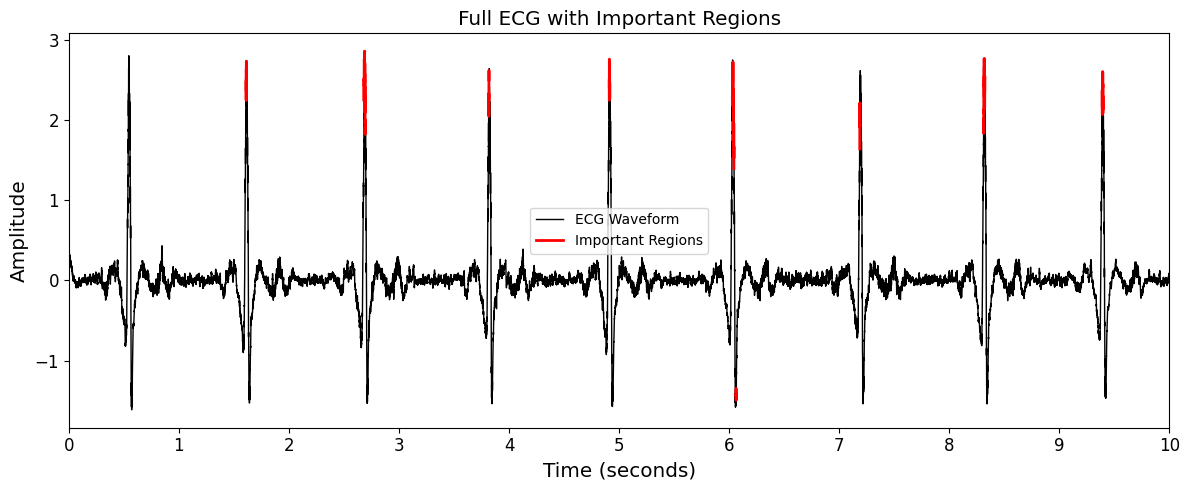
We interpret the fine-tuned model using the multimodal_signal_image_attribution interpretation method from PyKale, which builds on Captum’s Integrated Gradients to generate visual explanations for both CXR and ECG inputs. This method helps identify which regions in each modality, such as specific waveform segments in ECG and spatial regions in CXR, contributed most to the model’s prediction. This improves both transparency and clinical interpretability.

Estimated runtime: 10 seconds

from kale.interpret.signal_image_attribution import multimodal_signal_image_attribution
import matplotlib.pyplot as plt
import numpy as np

# User can change this to try different ECG and CXR interpretation configaration to play with
cfg_FT.INTERPRET.ECG_THRESHOLD = 0.75
cfg_FT.INTERPRET.SAMPLE_IDX = 3
cfg_FT.INTERPRET.ZOOM_RANGE = [3.5, 4]
cfg_FT.INTERPRET.CXR_THRESHOLD = 0.75


sample_idx = cfg_FT.INTERPRET.SAMPLE_IDX
zoom_range = tuple(cfg_FT.INTERPRET.ZOOM_RANGE)
ecg_threshold = cfg_FT.INTERPRET.ECG_THRESHOLD
cxr_threshold = cfg_FT.INTERPRET.CXR_THRESHOLD
lead_number = cfg_FT.MODEL.NUM_LEADS
sampling_rate = cfg_FT.INTERPRET.SAMPLING_RATE


# Run interpretation
result = multimodal_signal_image_attribution(
    last_fold_model=model_pl,
    last_val_loader=val_loader_FT,
    sample_idx=sample_idx,
    signal_threshold=ecg_threshold,
    image_threshold=cxr_threshold,
    zoom_range=zoom_range,
)

Full ECG View: Displays attribution across the full 12-lead ECG signal. A percentile-based threshold (e.g., top 25%) is applied to highlight segments with the highest contribution.

fig, ax = plt.subplots(figsize=(12, 5))
fig.patch.set_facecolor("white")
ax.set_facecolor("white")

# Plot the full ECG waveform
ax.plot(
    result["full_time"],
    result["signal_waveform_np"][: result["full_length"]],
    color="black",
    linewidth=1,
    label="ECG Waveform",
)

for idx in result["important_indices_full"]:
    stretch_start = max(0, idx - 6)
    stretch_end = min(result["full_length"], idx + 6 + 1)
    ax.plot(
        result["full_time"][stretch_start:stretch_end],
        result["signal_waveform_np"][stretch_start:stretch_end],
        color="red",
        linewidth=2,
    )

ax.set_xlabel("Time (seconds)", fontsize="x-large")
ax.set_ylabel("Amplitude", fontsize="x-large")
ax.set_title("Full ECG with Important Regions", fontsize="x-large")
ax.set_xticks(np.linspace(0, 10, 11))
ax.set_xlim([0, 10])
ax.tick_params(axis="x", labelsize="large")
ax.tick_params(axis="y", labelsize="large")
ax.legend(["ECG Waveform", "Important Regions"], fontsize="medium")

plt.tight_layout()
plt.show()

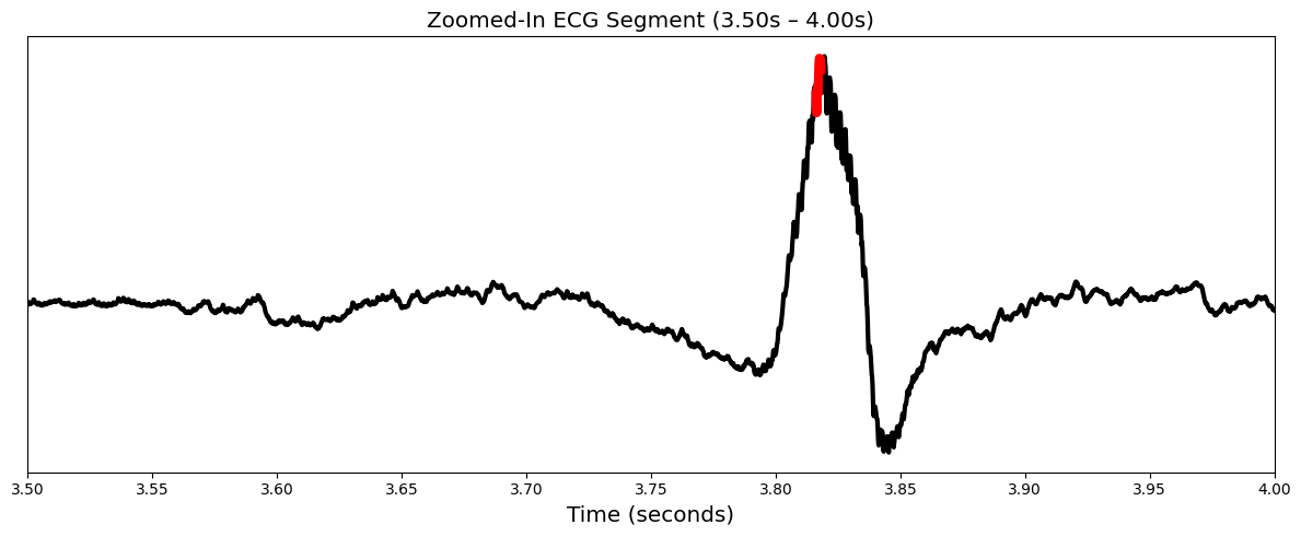
Zoomed-In ECG Segment: Focuses on a specific time window (e.g., 3 to 4 seconds) for fine-grained inspection of high-attribution waveform regions.

fig, ax = plt.subplots(figsize=(12, 5))
fig.patch.set_facecolor("white")
ax.set_facecolor("white")

# Plot zoomed-in ECG segment
ax.plot(
    result["zoom_time"],
    result["segment_signal_waveform"],
    color="black",
    linewidth=3,
    label="ECG Waveform",
)


for idx in result["important_indices_zoom"]:
    stretch_start = max(0, idx - 6)
    stretch_end = min(len(result["segment_signal_waveform"]), idx + 6 + 1)
    ax.plot(
        result["zoom_time"][stretch_start:stretch_end],
        result["segment_signal_waveform"][stretch_start:stretch_end],
        color="red",
        linewidth=6,
    )


ax.set_xticks(np.linspace(result["zoom_start_sec"], result["zoom_end_sec"], 11))
ax.set_xlim([result["zoom_start_sec"], result["zoom_end_sec"]])
ax.set_yticks([])
ax.set_xlabel("Time (seconds)", fontsize="x-large")
ax.set_ylabel("")
ax.set_title(
    f'Zoomed-In ECG Segment ({result["zoom_start_sec"]:.2f}s – {result["zoom_end_sec"]:.2f}s)',
    fontsize="x-large",
)

plt.tight_layout()
plt.show()

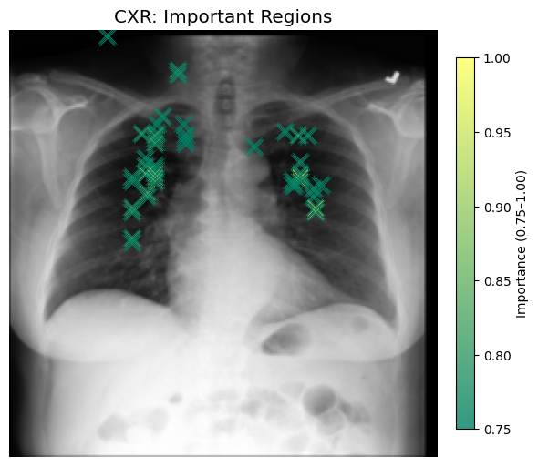
CXR Attribution Map: Shows a heatmap over the input CXR image, with highlighted areas corresponding to regions above a configurable percentile threshold (e.g., top 25%). This helps reveal where the model focused attention in the spatial domain.

x_pts = result["x_pts"]
y_pts = result["y_pts"]
importance_pts = result["importance_pts"]
cxr_thresh = result["image_threshold"]

fig, ax = plt.subplots(figsize=(6, 6))
fig.patch.set_facecolor("white")
ax.set_facecolor("white")

# Show base CXR image
ax.imshow(result["image_np"], cmap="gray", alpha=1)

# Overlay attribution points
sc = ax.scatter(
    x_pts,
    y_pts,
    c=importance_pts,
    cmap="summer",
    marker="x",
    s=150,
    vmin=cxr_thresh,
    vmax=1.0,
    alpha=0.8,
    linewidths=0.7,
    edgecolor="black",
)

# Add colorbar for importance
cbar = plt.colorbar(sc, ax=ax, fraction=0.04, pad=0.04)
cbar.set_label(f"Importance ({cxr_thresh:.2f}–1.00)")

# Final formatting
ax.axis("off")
ax.set_title("CXR: Important Regions", fontsize="x-large")

plt.tight_layout()
plt.show()

References

[1] Lu, H., Liu, X., Zhou, S., Turner, R., Bai, P., Koot, R. E., … & Xu, H. (2022, October). PyKale: Knowledge-aware machine learning from multiple sources in Python. In Proceedings of the 31st ACM International Conference on Information & Knowledge Management (pp. 4274-4278).

[2] Johnson, A., Pollard, T., Mark, R., Berkowitz, S., & Horng, S. (2024). MIMIC-CXR Database (version 2.1.0). PhysioNet. RRID:SCR_007345.

[3] Johnson, A. E., Pollard, T. J., Berkowitz, S. J., Greenbaum, N. R., Lungren, M. P., Deng, C. Y., … & Horng, S. (2019). MIMIC-CXR, a de-identified publicly available database of chest radiographs with free-text reports. Scientific data, 6(1), 317.

[4] Gow, B., Pollard, T., Nathanson, L. A., Johnson, A., Moody, B., Fernandes, C., Greenbaum, N., Waks, J. W., Eslami, P., Carbonati, T., Chaudhari, A., Herbst, E., Moukheiber, D., Berkowitz, S., Mark, R., & Horng, S. (2023). MIMIC-IV-ECG: Diagnostic Electrocardiogram Matched Subset (version 1.0). PhysioNet. RRID:SCR_007345.

[5] Suvon, M. N., Tripathi, P. C., Fan, W., Zhou, S., Liu, X., Alabed, S., … & Lu, H. (2024, October). Multimodal variational autoencoder for low-cost cardiac hemodynamics instability detection. In International Conference on Medical Image Computing and Computer-Assisted Intervention (pp. 296-306).