
Live-Coding Notebook#
Classification
Run cells on this page using the built-in Binder kernel, or open the notebook in Google Colab as an alternative. Colab requires additional dependency and companion-module setup.
Not connected. An interactive session starts only when you choose to launch it.
View on GitHub | Optional blank exercise | Execution help.
Sessions are temporary; save work you want to keep. Use synthetic data only: do not upload private or patient data. Synthetic results do not demonstrate clinical performance.
import torch
from IPython.display import display

from synthetic_data_generation import make_cohort
import pandas as pd

RANDOM_STATE = 0
0 Generate Synthetic Data#
data_folder = '../../../data/synthetic_data'
make_cohort(data_folder)
tabular_df = pd.read_csv(data_folder + '/clinical.csv', index_col=0)
display(tabular_df.head())
| age | gender | stage | |
|---|---|---|---|
| patient_id | |||
| patient_000 | 63.047171 | M | late |
| patient_001 | 49.600159 | F | early |
| patient_002 | NaN | F | early |
| patient_003 | 69.405647 | M | early |
| patient_004 | 40.489648 | F | early |
1 Data Loading#
1.1 Tabular#
from kalecancer.loaddata import Tabular

clinical_df = tabular_df.drop(columns =['stage'])

clinical_modality = Tabular(clinical_df)

# proof it works!
display(clinical_modality.frame.head())
display(clinical_modality['patient_000'])
display(clinical_modality.ids[:5])
display((clinical_modality.frame == clinical_df).any().any())
display((clinical_modality.ids == clinical_modality.frame.index).any())
display((clinical_df.index == clinical_modality.ids).any())
| age | gender | |
|---|---|---|
| id | ||
| patient_000 | 63.047171 | M |
| patient_001 | 49.600159 | F |
| patient_002 | NaN | F |
| patient_003 | 69.405647 | M |
| patient_004 | 40.489648 | F |
| age | gender | |
|---|---|---|
| id | ||
| patient_000 | 63.047171 | M |
Index(['patient_000', 'patient_001', 'patient_002', 'patient_003',
       'patient_004'],
      dtype='object', name='id')
np.True_
np.True_
np.True_
1.2 Patch Features#
Patch Features = Whole Slide Images passed through an encoder such as UNI
# What does the file structure look like
from pathlib import Path
list(Path(data_folder + '/patches').glob('*.h5'))[:5]
[PosixPath('../../../data/synthetic_data/patches/patient_027.h5'),
 PosixPath('../../../data/synthetic_data/patches/patient_082.h5'),
 PosixPath('../../../data/synthetic_data/patches/patient_057.h5'),
 PosixPath('../../../data/synthetic_data/patches/patient_044.h5'),
 PosixPath('../../../data/synthetic_data/patches/patient_026.h5')]
from kalecancer.loaddata import PatchFeatures

patch_features = PatchFeatures.from_glob(

    # 'what files are the patches stored in?'
    pattern = data_folder + '/patches/*.h5',

    # 'how to extract the ids from these files'
    id_pattern= r'(patient_\d{3})\.h5'
)

display(patch_features.ids[:5])
display(patch_features['patient_000'].shape)
display(patch_features['patient_000'].head())
Index(['patient_000', 'patient_001', 'patient_002', 'patient_003',
       'patient_004'],
      dtype='object', name='id')
(168, 35)
| file | x | y | feature_0 | feature_1 | feature_2 | feature_3 | feature_4 | feature_5 | feature_6 | ... | feature_22 | feature_23 | feature_24 | feature_25 | feature_26 | feature_27 | feature_28 | feature_29 | feature_30 | feature_31 | ||
|---|---|---|---|---|---|---|---|---|---|---|---|---|---|---|---|---|---|---|---|---|---|---|
| id | patch | |||||||||||||||||||||
| patient_000 | 0 | ../../../data/synthetic_data/patches/patient_0... | 26803 | 30774 | 3.152563 | 1.471492 | -2.566658 | -0.236850 | 0.176512 | 0.295994 | -0.371915 | ... | 0.438993 | 0.827988 | -0.296571 | 0.066546 | -0.697424 | 0.989584 | -1.178304 | 0.782350 | -0.190651 | 1.171247 |
| 1 | ../../../data/synthetic_data/patches/patient_0... | 25438 | 16956 | 3.750869 | 1.820646 | 0.730775 | -1.572040 | -0.066953 | -1.172007 | -0.518280 | ... | -2.063238 | -0.591103 | 0.590906 | -1.581594 | 1.475949 | 0.368357 | 0.846584 | -0.570944 | 0.813764 | 1.068472 | |
| 2 | ../../../data/synthetic_data/patches/patient_0... | 36345 | 43944 | 3.232878 | 0.234401 | 0.270343 | -0.863345 | -0.147529 | -0.152523 | 0.383394 | ... | -2.003522 | 1.604254 | -0.457699 | 0.107880 | 1.309551 | -1.602260 | -1.251647 | -1.601278 | -0.794136 | 0.439637 | |
| 3 | ../../../data/synthetic_data/patches/patient_0... | 35263 | 38608 | 3.524188 | 0.276274 | -1.412766 | -2.310103 | 0.054354 | -0.471776 | 0.459386 | ... | -1.296472 | -1.482185 | -2.333616 | -0.678264 | 0.749434 | -0.284884 | 0.197790 | 1.089218 | 1.327686 | -0.069138 | |
| 4 | ../../../data/synthetic_data/patches/patient_0... | 41517 | 18368 | 4.353586 | 0.092127 | -0.837398 | -0.594400 | -1.480536 | -0.888134 | -0.358017 | ... | 0.328662 | 0.361922 | 1.320662 | -0.342786 | -1.476858 | 1.067222 | -0.331488 | 1.114592 | 0.383377 | -0.131138 |
5 rows × 35 columns
1.3 The Target#
target_df = tabular_df['stage']
display(target_df.head(5))
patient_id
patient_000     late
patient_001    early
patient_002    early
patient_003    early
patient_004    early
Name: stage, dtype: object
from kalecancer.loaddata import Classification

target = Classification(labels=target_df, classes=['early', 'late'])
display(target.ids[:5])
display(target[['patient_000', 'patient_003']])
Index(['patient_000', 'patient_001', 'patient_002', 'patient_003',
       'patient_004'],
      dtype='object', name='id')
| label | |
|---|---|
| id | |
| patient_000 | late |
| patient_003 | early |
1.4 Multimodal Dataset: All Modalities Combined#
from kalecancer.loaddata import MultimodalDataset

dataset = MultimodalDataset(
    modalities={
       'clinical': clinical_modality,
       'wsi': patch_features
    },
    target=target,
    required_modalities=['clinical', 'wsi']
)

display(dataset.ids[:5])
display(dataset.summary())
display(dataset['patient_052'].keys())
display(dataset['patient_052']['clinical'])
Index(['patient_000', 'patient_001', 'patient_002', 'patient_003',
       'patient_004'],
      dtype='object', name='id')
| count | |
|---|---|
| available: clinical | 100 |
| available: wsi | 100 |
| available: target | 100 |
| included | 100 |
| included with clinical | 100 |
| included with wsi | 100 |
| label: early | 53 |
| label: late | 47 |
dict_keys(['clinical', 'wsi', 'target'])
| age | gender | |
|---|---|---|
| id | ||
| patient_052 | NaN | F |
2 Model Building#
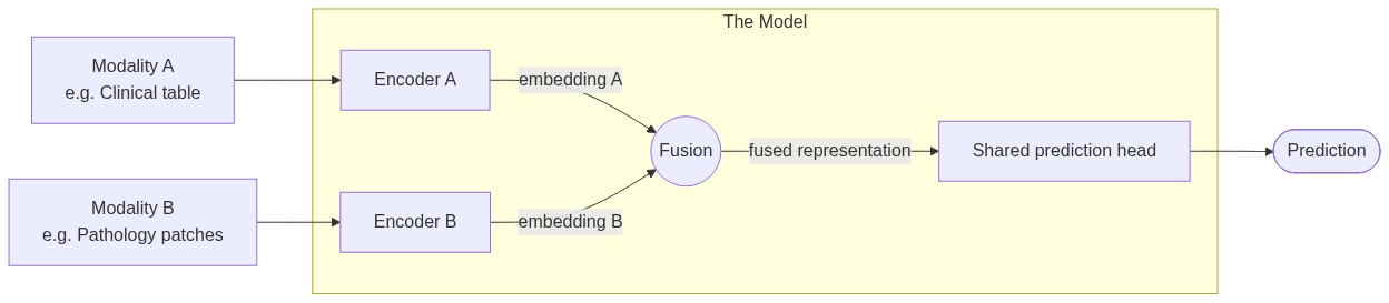
2.1 Intermediate Fusion#
import base64
from IPython.display import Image, display

graph = """
flowchart LR
    A[Modality A<br/>e.g. Clinical table] --> EA
    B[Modality B<br/>e.g. Pathology patches] --> EB
    subgraph M[The Model]
        EA[Encoder A]
        EB[Encoder B]
        F((Fusion))
        H[Shared prediction head]
        EA -->|embedding A| F
        EB -->|embedding B| F
        F -->|fused representation| H
    end
    H --> O([Prediction])
"""

encoded = base64.urlsafe_b64encode(graph.encode()).decode()
display(Image(url=f"https://mermaid.ink/img/{encoded}"))
# Needed to ensure model weights are initialised consistently
torch.manual_seed(RANDOM_STATE)
<torch._C.Generator at 0x7dd0081f4650>
from kalecancer.model import ABMIL, IntermediateFusion, Concat, ClassificationHead

inter_model = IntermediateFusion(
    encoders = {
        'clinical': [torch.nn.Linear(dataset.modalities['clinical'].frame.shape[1], 8)],
        'wsi': [
            ABMIL(32, hidden_dim=16, attention_dim=8, dropout=0.0),
            torch.nn.Linear(16,8)
        ]
    },

    # the encoder outputs concatenated
    fusion = Concat(),

    head = ClassificationHead(in_dim=16, n_classes=2)
)
display(inter_model.modalities)
display(inter_model.encoders['clinical'])
display(inter_model.encoders['wsi'])
display(inter_model.fusion)
display(inter_model.head)
['clinical', 'wsi']
EncoderList(
  (0): Linear(in_features=2, out_features=8, bias=True)
)
EncoderList(
  (0): ABMIL(
    (embed): Sequential(
      (0): Linear(in_features=32, out_features=16, bias=True)
      (1): ReLU()
      (2): Dropout(p=0.0, inplace=False)
    )
    (attention_value): Sequential(
      (0): Linear(in_features=16, out_features=8, bias=True)
      (1): Tanh()
    )
    (attention_gate): Sequential(
      (0): Linear(in_features=16, out_features=8, bias=True)
      (1): Sigmoid()
    )
    (attention_score): Linear(in_features=8, out_features=1, bias=True)
  )
  (1): Linear(in_features=16, out_features=8, bias=True)
)
Concat()
ClassificationHead(
  (linear): Linear(in_features=16, out_features=2, bias=True)
)
3 The Model Orchestrator#
3.1 Creating the Transformation#
Trained/fitted transforms must be passed into the Pipeline object, and not applied beforehand.
Training/fitting transforms on the full dataset (train + test) is data leakage!
# getting insight into the tabular data, needed to understand what transforms to apply
print('Number of missing values:')
display(dataset.modalities['clinical'].frame.isna().sum())
print('\nNumber unique values:')
display(dataset.modalities['clinical'].frame.nunique())
Number of missing values:
age       10
gender     8
dtype: int64
Number unique values:
age       90
gender     2
dtype: int64
dataset['patient_002']['clinical']
| age | gender | |
|---|---|---|
| id | ||
| patient_002 | NaN | F |
# from the above information we make must make the following transforms.
from sklearn.preprocessing import StandardScaler, OrdinalEncoder
from sklearn.impute import SimpleImputer
from sklearn.compose import ColumnTransformer
from sklearn.pipeline import make_pipeline

numeric_pipeline = make_pipeline(SimpleImputer(), StandardScaler())

tab_transfromers = ColumnTransformer([
    ('numeric', numeric_pipeline, ['age']),
    ('categorical', OrdinalEncoder(encoded_missing_value=-1), ['gender'])
])
3.2 Creating the Orchestrator: Pipeline#
from kalecancer.pipeline import Pipeline
from functools import partial

pipeline = Pipeline(
    model= inter_model,

    # these are transforms that will be applied to the dataset
    # currently only Tabular modalities accept transforms
    # transforms need to ouptut numerical values, and their output should be
    # accepted by the first encoder
    transforms={'clinical': tab_transfromers},

    optimizer= partial(torch.optim.AdamW, lr=1e-3),
    batch_size=32,
    drop_last=True,
    max_epochs=40,
    validation=None,
    early_stopping=None,
    accelerator='cpu',
    precision='32-true',
    random_state=RANDOM_STATE,
)
4 Training#
4.1 Fitting#
from kalecancer.loaddata import train_test_split
train, test = train_test_split(dataset, test_size=0.2, stratify=True, random_state=RANDOM_STATE)

display(len(train))
display(len(test))
80
20
pipeline.fit(train)
Pipeline(accelerator='cpu', batch_size=32, drop_last=True, early_stopping=None,
         max_epochs=40,
         model=IntermediateFusion(
  (encoders): ModuleDict(
    (clinical): EncoderList(
      (0): Linear(in_features=2, out_features=8, bias=True)
    )
    (wsi): EncoderList(
      (0): ABMIL(
        (embed): Sequential(
          (0): Linear(in_features=32, out_features=16, bias=True)
          (1): ReLU()
          (2): Dropout(p=0.0, inplace=Fals...
         optimizer=functools.partial(<class 'torch.optim.adamw.AdamW'>, lr=0.001),
         precision='32-true', random_state=0,
         transforms={'clinical': ColumnTransformer(transformers=[('numeric',
                                                                  Pipeline(steps=[('simpleimputer',
                                                                                   SimpleImputer()),
                                                                                  ('standardscaler',
                                                                                   StandardScaler())]),
                                                                  ['age']),
                                                                 ('categorical',
                                                                  OrdinalEncoder(encoded_missing_value=-1),
                                                                  ['gender'])])},
         validation=None)
In a Jupyter environment, please rerun this cell to show the HTML representation or trust the notebook. On GitHub, the HTML representation is unable to render, please try loading this page with nbviewer.org.
Parameters
| model | IntermediateF...as=True) ) ) | |
| transforms | {'clinical': ColumnTransfo... ['gender'])])} | |
| optimizer | functools.par...W'>, lr=0.001) | |
| batch_size | 32 | |
| drop_last | True | |
| max_epochs | 40 | |
| validation | None | |
| early_stopping | None | |
| accelerator | 'cpu' | |
| precision | '32-true' | |
| random_state | 0 | |
| param_groups | None | |
| num_workers | 0 | |
| trainer_kwargs | None |
Fitted attributes
| Name | Type | Value |
|---|---|---|
| baseline_ | NoneType | None |
| fit_report_ | dict | {'be...ch': None, 'be...re': None, 'ep...un': 40, 'la...ly': 42, ...} |
| history_ | DataFrame | train_... 0 |
| model_ | IntermediateFusion | IntermediateF...as=True) ) ) |
| target_ | Classification | <kalecancer.l...x7dce89b21fa0> |
| train_ids_ | list | ['pa...00', 'pa...02', 'pa...03', 'pa...06', ...] |
| train_target_ | DataFrame | ...s x 1 columns] |
| transforms_ | dict | {'cl...al': ColumnTransfo... ['gender'])])} |
| val_ids_ | list | [] |
display(pipeline.history_.head())
| train_loss | optimizer_steps | skipped_batches | |
|---|---|---|---|
| epoch | |||
| 0 | 0.693046 | 2 | 0 |
| 1 | 0.698229 | 4 | 0 |
| 2 | 0.708995 | 6 | 0 |
| 3 | 0.693900 | 8 | 0 |
| 4 | 0.701664 | 10 | 0 |
4.2 [OPTIONAL] How are the transformers fitted?#
# [OPTIONAL]
# Insight into how the transformers are applied in the Pipeline.fit

fitted_t = tab_transfromers.fit(train.modalities['clinical'].frame)
fitted_train = train.modalities['clinical'].with_transform(fitted_t, train.ids)

print('Number of missing values before transforms:')
print(train.modalities['clinical'].frame.isna().sum().sum())

print()
print('Number of missing values after transforms:')
print(fitted_train.frame.isna().sum().sum())
Number of missing values before transforms:
18

Number of missing values after transforms:
0
5 Evaluation#
Note that we are using small synthetic illustrative cohort, so results don’t provide real clinical insight
5.1 Prediction#
pipeline.predict(test).head()
| probability[early] | probability[late] | |
|---|---|---|
| id | ||
| patient_001 | 0.552869 | 0.447131 |
| patient_004 | 0.652484 | 0.347516 |
| patient_005 | 0.573326 | 0.426674 |
| patient_012 | 0.533786 | 0.466215 |
| patient_013 | 0.431970 | 0.568030 |
5.2 Evaluation#
from kalecancer.evaluate import AUROC, BalancedAccuracy
pipeline.evaluate(test, metrics={"auroc": AUROC(positive_class='late'), "balanced_acc": BalancedAccuracy()})
auroc           0.727273
balanced_acc    0.631313
Name: score, dtype: float64
6 [Advanced] Comparing Models#
from kalecancer.model import Unimodal
from sklearn.base import clone
torch.manual_seed(0)
clinical_model = Unimodal(
    "clinical",
    encoders=[torch.nn.Linear(dataset.modalities['clinical'].frame.shape[1], 8)],
    head=ClassificationHead(in_dim=8, n_classes=2),
)
baseline_pipeline = clone(pipeline).set_params(model=clinical_model).fit(train)
from kalecancer.evaluate import EvalContext, bootstrap_ci
prediction, baseline_prediction = pipeline.predict(test), baseline_pipeline.predict(test)

target = test.target.frame.loc[prediction.index]
context = EvalContext(train_target=pipeline.train_target_, classes=pipeline.target_.classes)
baseline_context = EvalContext(train_target=baseline_pipeline.train_target_, classes=baseline_pipeline.target_.classes)

intervals = {
    "fused": bootstrap_ci( AUROC(positive_class='late'), prediction, target, context),
    "clinical only": bootstrap_ci( AUROC(positive_class='late'), baseline_prediction, target, baseline_context),
    "gain from the slides": bootstrap_ci(
         AUROC(positive_class='late'), prediction, target, context, baseline=baseline_prediction, baseline_context=baseline_context
    ),
}
table = pd.DataFrame({name: vars(ci) for name, ci in intervals.items()}).T[["estimate", "lower", "upper"]]
# explicit, as not every editor renders a bare DataFrame on the last line (PyCharm, for one)
display(table)
| estimate | lower | upper | |
|---|---|---|---|
| fused | 0.727273 | 0.484706 | 0.939394 |
| clinical only | 0.626263 | 0.353535 | 0.875000 |
| gain from the slides | 0.101010 | -0.046966 | 0.250000 |